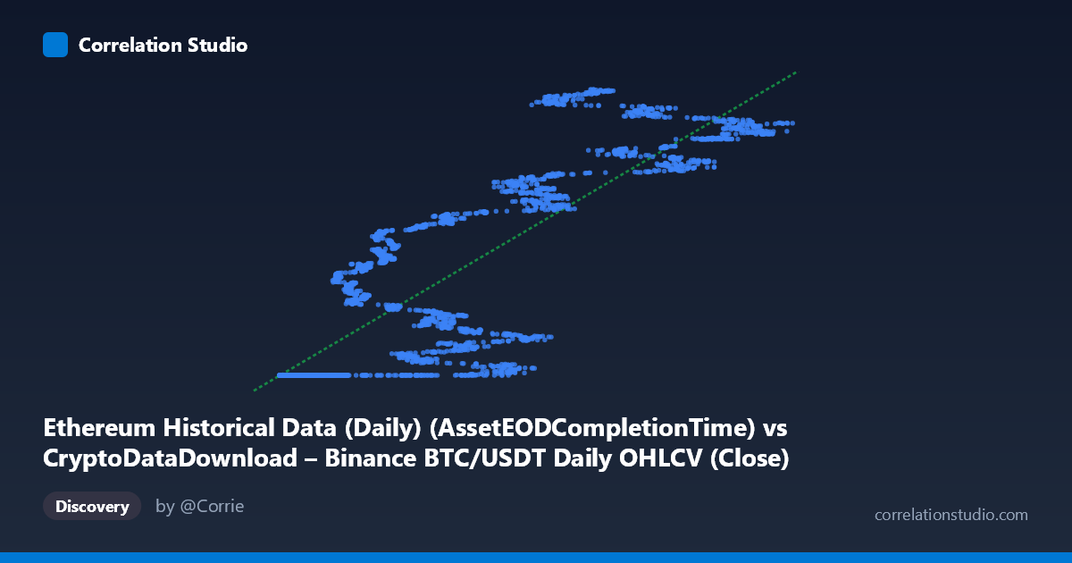
Ethereum Historical Data (Daily) (AssetEODCompletionTime) vs CryptoDataDownload – Binance BTC/USDT Daily OHLCV (Close)

Pearson correlation (r): 0.8523
Spearman correlation: 0.8876
p-value: 0
Sample size (n): 3191
95% confidence interval: 0.8425 to 0.8615
Granger causality: None
Granger optimal lag: 10

AI analysis

Analysis of BTC/USDT–ETH Price Relationship

1. Overview of the Relationship

The scatterplot displays a strong positive association between the X variable (mislabeled in the column header but numerically resembling a small-denomination metric, likely an EOD completion time or price parameter) and Y (BTC/USDT daily close price). As X increases, Y trends upward in a broadly linear, though not perfectly smooth, fashion. The data show a distinctive floor effect: for X values below roughly 25,000, Y clusters tightly near 1,614,335,000–1,614,336,000, suggesting a saturated or capped minimum price regime before the relationship "activates" and begins scaling upward with X.

2. Correlation Strength, Variance Explained, and Causality

The Pearson correlation of r = 0.852 indicates a strong positive linear relationship, and r² = 0.727 means about 72.7% of the variance in Y is statistically explained by X — a substantial but not complete accounting, leaving over a quarter of Y's variance driven by other factors or nonlinearities. The 95% CI [0.843, 0.862] is narrow, reflecting high confidence in the correlation estimate given the large sample (n=3,191), and the p-value of ~0 confirms this relationship is highly unlikely due to chance. However, the Granger causality tests (optimal lag = 10 periods) show no significant predictive direction in either direction (X→Y: p=0.33; Y→X: p=0.17). This is a critical caveat: despite strong contemporaneous correlation, neither series reliably predicts the other's future movements at this lag structure — the relationship may be driven by a shared underlying trend (e.g., both tracking overall crypto market cycles) rather than one causally leading the other.

3. Notable Patterns and Outliers

The most visually striking feature is the plateau: dozens of points with X < 25,000 all map to nearly identical Y values (~1.614 billion), forming a dense horizontal cluster at the low end. This suggests either a data artifact (e.g., a placeholder/minimum value during an early period, possibly reflecting BTC's actual price floor around $16,143 if scaled correctly), a market floor during a specific time window, or truncation/rounding in the data source. Above X≈25,000, the relationship becomes more dispersed and heteroscedastic — variance in Y increases with X, and secondary clustering appears around X=60,000–85,000 with Y values spanning 1.70–1.78 billion, hinting at distinct market regimes or volatility phases (e.g., bull-market accelerations) rather than a single smooth linear trend.

4. Confounding Factors and Caveats

Several caveats merit attention. First, both BTC and ETH prices are known to be highly autocorrelated and jointly driven by macro crypto-market sentiment, liquidity, and regulatory news — a classic confounding structure that inflates correlation without implying direct causal linkage. Second, the flat cluster at low X values (spanning what appears to be an extended date range from 2017 onward) may reflect a specific historical period (e.g., 2017–2019 bear/accumulation phase) where BTC price was essentially rangebound, artificially inflating the linear fit's apparent strength once combined with the later high-X, high-Y bull period — a scenario prone to spurious correlation from shared time trends. Third, mismatched or mislabeled axis metadata (X axis described as "AssetEODCompletionTime" but behaving like a price/volume metric) raises data-integrity concerns that should be resolved before drawing strong conclusions.

5. Recommendations for Further Investigation

To strengthen this analysis: (a) verify and correct the column labeling/units for the X variable, since "completion time" is an unusual driver of price; (b) de-trend both series (e.g., using returns or log-differences rather than levels) and re-run correlation/Granger tests, since price levels are non-stationary and prone to spurious regression; (c) segment the data by the identified low-X plateau period versus the dispersed high-X period to test whether the relationship holds within regimes or is an artifact of pooling two structurally different eras; and (d) given the null Granger causality result, consider testing alternative lag structures, or a cointegration/error-correction model, to properly characterize any lead-lag dynamics obscured by simple linear correlation on raw price levels.

X dataset: CryptoDataDownload – Binance BTC/USDT Daily OHLCV

Y dataset: Ethereum Historical Data (Daily)

Part of experiment: Bitcoin - CryptoDataDownload – Binance BTC/USDT Daily OHLCV vs Ethereum Historical Data (Daily)