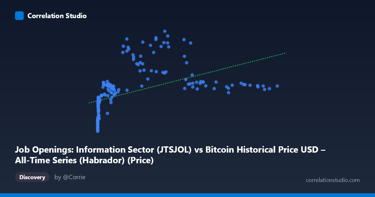
Job Openings: Information Sector (JTSJOL) vs Bitcoin Historical Price USD – All-Time Series (Habrador) (Price)
- Pearson correlation (r)
- 0.4926
- Spearman correlation
- 0.8642
- p-value
- 0
- Sample size (n)
- 189
- 95% confidence interval
- 0.3764 to 0.5936
- Granger causality
- None
- Granger optimal lag
- 10
AI analysis
Analysis: Bitcoin Price vs. Information Sector Job Openings
1. What the Visualization Reveals
The scatterplot shows a positive but noisy relationship between Bitcoin's historical price (X-axis, spanning an enormous range from $0.06 to $118,670) and monthly job openings in the Information sector (Y-axis, ranging from ~2,918 to 12,301). The data reveals a clear non-linear pattern: at very low Bitcoin prices (under $1,000), job openings cluster tightly in the 3,000–6,000 range, while as Bitcoin prices climb into the tens of thousands, job openings become both higher on average and much more scattered (ranging from ~6,500 to over 12,000). This fan-shaped dispersion suggests heteroscedasticity rather than a clean linear trend.
2. Strength, Direction, and Predictive Value
The Pearson correlation (r = 0.493) indicates a moderate positive relationship, but r² = 0.243 means only about 24% of the variance in job openings is explained by Bitcoin price — leaving roughly 76% unexplained. The 95% CI [0.376, 0.594] is reasonably tight and excludes zero, and the p-value (6×10⁻¹³) confirms this correlation is highly statistically significant and not due to chance, even with n=189. However, statistical significance here reflects the large sample size more than practical predictive strength — a moderate r with a huge N will always be "significant." Critically, the Granger causality tests (both directions non-significant, p 0.59) show no evidence that either variable temporally predicts the other. This strongly suggests the correlation is not causal in either direction but likely reflects both series independently trending upward over the same 2010–2026 period (i.e., a shared time trend or spurious correlation from co-occurring macro cycles).
3. Notable Patterns and Outliers
Several features stand out: (a) a dense cluster of low-X, low-Y points representing Bitcoin's early years (2010–2013) where prices were near-zero and job openings were also comparatively low (~3,000–4,000); (b) increasing scatter/variance at higher Bitcoin prices — e.g., at X≈45,000–60,000 Y ranges from 6,943 to 12,301, showing no consistent Y value for similar X; (c) a notable outlier at (44,354.64, 12,301) — the maximum Y value paired with a mid-range X, breaking any clean trend; and (d) at very high X (85,000), Y actually drops back to 6,500–7,600, contradicting a monotonic relationship and hinting at a possible peak-and-decline or non-monotonic pattern (consistent with Bitcoin's 2021 peak followed by a 2022 crash while job openings may have moved on a different cycle).
4. Confounding Factors and Caveats
This is a textbook case of two time series being compared without controlling for their shared temporal trend. Both Bitcoin price and Information-sector job openings grew substantially over 2010–2026 due to entirely different macro drivers — Bitcoin due to speculative adoption cycles, job openings due to broader tech-sector labor market growth (partly independent of crypto). Neither variable has an obvious causal mechanism linking it to the other; any correlation is almost certainly confounded by omitted variables such as overall economic growth, monetary policy (low interest rates fueling both tech hiring and speculative asset bubbles), or simple time-trend co-movement. The extreme right-skew of X (mean 20,533 vs. median likely much lower, given the range) also means a few large Bitcoin price observations could be disproportionately influencing the linear fit.
5. Actionable Insights
Given the lack of Granger causality and the note that Spearman ρ exceeds Pearson r, analysts should treat this correlation as spurious/trend-driven rather than predictive. Recommended next steps: (1) detrend both series (e.g., first-difference or year-over-year % change) and re-test correlation to see if it disappears — this would confirm the relationship is trend-driven; (2) test a log-transform of X (given its extreme range and the log-like hint from Spearman/Pearson divergence), which may reveal a more linear log(X) vs. Y relationship; (3) introduce a proper macroeconomic control (e.g., Fed funds rate, NASDAQ index, or overall labor market tightness) to see if it explains both series jointly; and (4) avoid using Bitcoin price as a leading indicator for tech-sector hiring decisions, as the Granger test provides no support for such a use case.
X dataset: Bitcoin Historical Price USD – All-Time Series (Habrador)
Y dataset: Job Openings: Information Sector
Part of experiment: Bitcoin - Bitcoin Historical Price USD – All-Time Series (Habrador) vs Job Openings: Information Sector