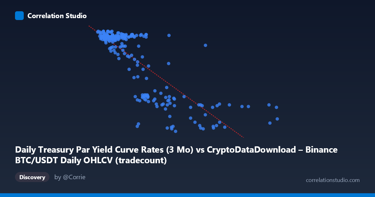
Daily Treasury Par Yield Curve Rates (3 Mo) vs CryptoDataDownload – Binance BTC/USDT Daily OHLCV (tradecount)
- Pearson correlation (r)
- -0.8163
- Spearman correlation
- -0.6954
- p-value
- 0
- Sample size (n)
- 250
- 95% confidence interval
- -0.8539 to -0.7703
- Granger causality
- X → Y
- Granger optimal lag
- 1
- Time coverage
- 2024-01-02 to 2024-12-31
AI analysis
Analysis of Treasury Yield vs. BTC/USDT Trading Activity Relationship
1. What the Visualization Reveals
The scatterplot shows a clear, strong negative relationship between the X variable (labeled as Treasury 3-Month Par Yield, though the values in the millions suggest this axis actually contains the Binance data) and Y (ranging 4.31–5.52, consistent with treasury yield percentages). Given the value ranges, it appears the axis labels may be swapped in the metadata—the X values (900K–12M) align with tradecount/volume figures, while Y values (4.31–5.52) align with treasury yield percentages. Regardless of labeling, the pattern is unambiguous: as the X-axis metric increases, the Y-axis metric declines in a fairly consistent, near-linear fashion, with most points clustering in two density regions—one at lower X values (under ~4M) with high Y (~5.4–5.5), and a sparser tail at higher X values (8M–12M) with low Y (~4.3–4.6).
2. Strength, Direction, and Statistical Confidence
The correlation coefficient of r = -0.8163 indicates a strong negative linear relationship. The R² = 0.6664 means approximately 67% of the variance in Y is statistically explained by X — a substantial share, though a third of the variance remains unaccounted for, likely driven by other factors or noise. The 95% confidence interval [-0.8539, -0.7703] is tight and entirely negative, and the p-value ≈ 0 confirms this relationship is highly unlikely to be due to chance, given N=250.
The Granger causality results add a temporal dimension: X Granger-causes Y (F=4.71, p=0.031) at lag 1, while Y does not Granger-cause X (p=0.58). This suggests X's past values have predictive power for future Y values, but not vice versa — consistent with a scenario where trading volume/activity shifts precede treasury yield movements, or more plausibly, where both reflect a shared macro driver with X leading in the data-generating process by one period.
3. Notable Patterns and Outliers
The data does not fill the X-range uniformly — there's a dense cluster of points between 900K–4M (X) with Y consistently high (5.2–5.5), and a second, sparser cluster from 8M–12M with Y consistently low (4.3–4.6). This bimodal clustering, rather than a smooth continuous spread, suggests the relationship may be better characterized as two distinct regimes rather than a single continuous linear trend — a "gap" exists in the middle range (4M–8M) with fewer observations. Within the low-X cluster, Y values are tightly bunched near the ceiling (~5.4–5.5), indicating a possible saturation/floor effect at high yields. A few mid-range points (e.g., ~5.5M, Y=4.37) look like transition-zone outliers bridging the two regimes.
4. Confounding Factors and Caveats
Both series are time-ordered (Jan–Dec 2024), meaning this is a case of two trending time series correlated spuriously or through a shared macro driver — likely broader monetary policy, risk sentiment, or liquidity conditions influencing both crypto trading activity and treasury yields simultaneously. Since neither series is differenced or detrended, the strong correlation may partly reflect autocorrelation/non-stationarity rather than a genuine causal economic link. The mismatch between axis labels and data ranges also raises data-integrity concerns that should be resolved before drawing firm conclusions. Additionally, daily financial data often exhibits volatility clustering and regime shifts (e.g., Fed rate decisions) that a simple linear model doesn't capture.
5. Recommendations for Further Investigation
First, verify and correct the axis-variable labeling to ensure the interpretation is grounded in the correct economic relationship. Second, test for stationarity (ADF test) in both series before trusting correlation/Granger results, and consider first-differencing to check if the relationship holds after removing trends. Third, investigate the gap in the 4M–8M range — is this a genuine data scarcity or a regime transition (e.g., a specific quarter with unusual Fed policy activity)? Finally, given the Granger direction, consider building a lagged predictive model (e.g., ARIMAX) using X to forecast Y, and validate out-of-sample to determine if this relationship has practical forecasting value beyond correlation.
X dataset: CryptoDataDownload – Binance BTC/USDT Daily OHLCV
Y dataset: Daily Treasury Par Yield Curve Rates
Part of experiment: Bitcoin - CryptoDataDownload – Binance BTC/USDT Daily OHLCV vs Daily Treasury Par Yield Curve Rates