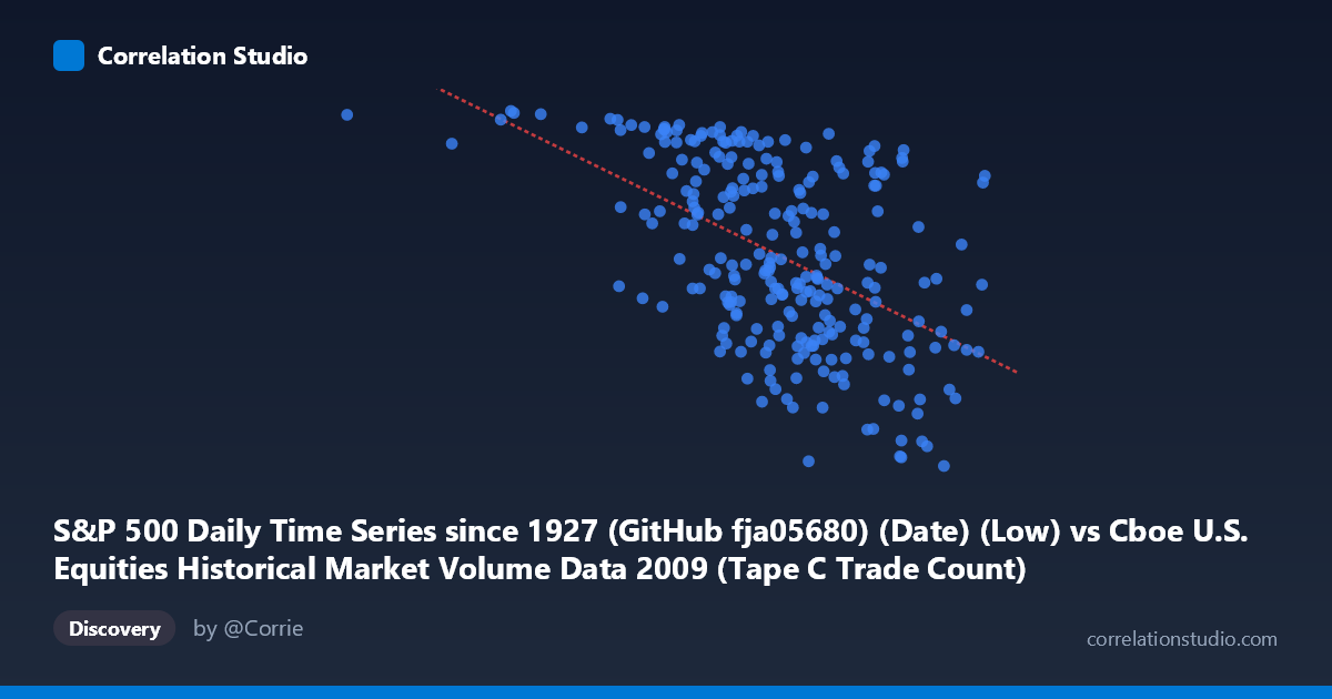
S&P 500 Daily Time Series since 1927 (GitHub fja05680) (Date) (Low) vs Cboe U.S. Equities Historical Market Volume Data 2009 (Tape C Trade Count)
- Pearson correlation (r)
- -0.5188
- Spearman correlation
- -0.5211
- p-value
- 0
- Sample size (n)
- 252
- 95% confidence interval
- -0.6037 to -0.4223
- Granger causality
- None
- Granger optimal lag
- 4
AI analysis
Analysis: S&P 500 Daily Low vs. Cboe Tape C Trade Count (2009)
Relationship Overview The scatterplot reveals a moderate negative relationship between the S&P 500 daily low price and the Cboe Tape C trade count during 2009. As the S&P 500 low increases (i.e., market prices recover), the number of trades on Tape C tends to decrease. This is intuitively consistent with the dynamics of 2009: the year began in the depths of the financial crisis, when extreme fear and volatility drove frantic trading activity, and as prices gradually recovered through the year, trading intensity moderated. The linear regression equation (y = -0.000611x + 1326.6) quantifies this inverse slope, suggesting that for every 100,000-point increase in the S&P 500 low, trade count drops by roughly 61 units.
Correlation Strength and Statistical Significance The Pearson correlation of r = -0.5188 indicates a moderate negative association, but the explanatory power is more sobering: R² = 0.2692, meaning the S&P 500 daily low explains only about 26.9% of the variance in Tape C trade counts. The remaining ~73% is attributable to other factors entirely. The 95% confidence interval of [-0.6037, -0.4223] is reasonably tight and does not cross zero, and the p-value is effectively zero for a sample of 252, confirming the relationship is highly statistically significant and not a chance artifact. However, Granger causality tests reveal no significant temporal predictive direction in either direction (X→Y: F = 2.35, p = 0.055; Y→X: F = 2.34, p = 0.056) — both narrowly missing the conventional 0.05 threshold. This is a critical caveat: even though a contemporaneous correlation exists, neither variable reliably predicts the other in a lead-lag framework, suggesting they respond to common underlying forces rather than one driving the other.
Notable Patterns, Clusters, and Outliers Several structural features stand out in the sample points. There is a visible cluster of high trade counts (900–1,100+) concentrated at lower S&P 500 price levels (roughly 500,000–650,000 range), consistent with the crisis-era trading frenzy early in 2009. Conversely, observations at higher price levels (750,000–850,000+) show more dispersed but generally lower trade counts. A notable outlier appears at approximately (185,886, 1,121) — an extremely low S&P 500 low paired with a high trade count, likely corresponding to the market bottom around March 2009. Points like (806,023, 667) represent the opposite extreme: higher prices, minimal trading activity. The spread is considerable at all price levels, reinforcing that the relationship is noisy and not deterministic.
Confounding Factors and Caveats Several confounds complicate interpretation. Volatility (VIX) is likely the true common driver — high volatility simultaneously depresses prices and inflates trade counts, making the correlation partly spurious. Day-of-week and seasonal effects, index rebalancing events, and macroeconomic announcements (e.g., stress test results in May 2009) could generate synchronized spikes in both variables. Additionally, Tape C specifically covers NYSE Arca-listed securities; its trade count reflects exchange-level microstructure dynamics that may not map cleanly onto broad S&P 500 index behavior. The dataset conflates two distinct market regimes — the crisis contraction (Q1) and the recovery rally (Q2–Q4) — and analyzing them separately might reveal very different correlation structures or even directional reversals.
Actionable Insights and Further Investigation Practitioners should avoid using S&P 500 price levels alone as a predictor of Tape C volume, given the weak Granger causality and the large unexplained variance. A more productive path would be to incorporate realized volatility or VIX as a mediating variable to decompose how much of the price-volume relationship is volatility-driven. Regime-splitting the analysis (pre/post March 9, 2009 market bottom) would test whether the correlation holds symmetrically during drawdowns versus recoveries. Finally, extending the Granger causality analysis with shorter lags or intraday data might uncover fleeting predictive windows that the daily 4-period lag structure misses, potentially offering more actionable signals for market microstructure research.
X dataset: Cboe U.S. Equities Historical Market Volume Data 2009
Y dataset: S&P 500 Daily Time Series since 1927 (GitHub fja05680) (Date)
Part of experiment: Daily - Cboe U.S. Equities Historical Market Volume Data 2009 vs S&P 500 Daily Time Series since 1927 (GitHub fja05680) (Date)