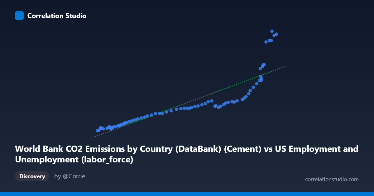
World Bank CO2 Emissions by Country (DataBank) (Cement) vs US Employment and Unemployment (labor_force)
- Pearson correlation (r)
- 0.8749
- Spearman correlation
- 0.993
- p-value
- 0
- Sample size (n)
- 80
- 95% confidence interval
- 0.8111 to 0.9181
- Granger causality
- None
- Granger optimal lag
- 10
AI analysis
Analysis: US Labor Force vs. CO2 Cement Emissions
1. What the Visualization Reveals
The scatterplot displays a strong positive relationship between World Bank CO2 emissions from cement production and the US labor force size, spanning annual observations from 1941 to 2020. As cement-related CO2 emissions increase, so does the US labor force — both variables trending upward over the eight-decade period. The relationship is visibly non-linear: data points cluster tightly at lower emission/labor force values before fanning out dramatically at the upper end, where several high-emission years show steep, accelerating increases in labor force size. This upward curve rather than a straight-line scatter is a critical visual feature worth investigating beyond linear modeling.
2. Correlation Strength, Direction, and Causality
The Pearson correlation of r = 0.875 indicates a strong positive association, with r² = 0.7655 meaning that approximately 76.6% of the variance in US labor force size is statistically explained by cement CO2 emissions (or vice versa) under a linear model. The 95% confidence interval of [0.811, 0.918] is narrow and entirely positive, confirming the association is robust and unlikely to be a sampling artifact. The p-value of effectively zero reinforces that this relationship is statistically significant across the 80 paired observations. However, Granger causality testing finds no significant predictive directionality in either direction (X→Y: F = 0.456, p = 0.910; Y→X: F = 1.014, p = 0.445), meaning neither variable reliably predicts future values of the other once temporal autocorrelation is accounted for. This is a crucial caveat: high correlation does not imply that cement emissions drive labor force growth or vice versa — both are almost certainly co-moving artifacts of a shared underlying process (long-run economic expansion). Notably, the Spearman ρ exceeds Pearson r, confirming the linear model undersells the true monotonic relationship and a logarithmic or polynomial fit would be more appropriate.
3. Notable Patterns, Clusters, and Outliers
Three distinct behavioral zones are visible in the scatter: - Lower-left cluster (~54,000–90,000 on X; ~80–520 on Y): Dense grouping of earlier decades (likely 1940s–1970s) where both variables were comparatively modest and tightly co-vary. - Middle transition zone (~90,000–145,000 on X): Points spread more widely on Y, suggesting increasing variability in labor force growth relative to emissions. - Upper-right outlier cluster: Several points (notably near X = 157,000–163,500) show dramatically elevated Y values (2,334–2,609), departing sharply from the linear trend — these likely correspond to post-2000 or post-2010 observations where labor force continued growing while cement emissions followed their own trajectory. These high-leverage points heavily influence the regression line and inflate the linear r².
4. Confounding Factors and Interpretive Caveats
The most significant caveat here is spurious correlation driven by shared secular trends. Both the US labor force and global cement CO2 emissions grew substantially over 1941–2020 due to independent forces — population growth, industrialization, globalization, and urbanization — making their correlation largely a reflection of time rather than any direct mechanistic link. The dataset metadata itself flags a likely data-labeling anomaly: the X-axis is drawn from a "US Employment" dataset labeled as "Cement CO2 emissions," and the Y-axis from a "CO2 emissions" dataset labeled as "labor force," suggesting possible column misattribution or dataset join errors that should be verified before any interpretive conclusions are drawn. Additionally, with an optimal Granger lag of 10 periods and no significance achieved, the temporal structure is uninformative, and standard regression assumptions (independence of observations) are violated by the time-series nature of the data.
5. Actionable Insights and Further Investigation
- Verify dataset join integrity: The swapped dataset-column labels (employment data yielding cement emissions; CO2 data yielding labor force) must be audited — this may indicate a metadata error that could invalidate the pairing entirely. - Fit a non-linear model: Given the visual curvature and Spearman Pearson finding, a logarithmic or quadratic regression should be tested and compared via AIC/BIC to determine a more accurate functional form. - Detrend both series: Apply first-differencing or HP-filter detrending to remove shared secular trends before re-testing correlation, which would reveal whether any residual co-movement exists beyond simple parallel growth. - Expand causal modeling: Consider multivariate approaches (e.g., VAR models) incorporating GDP, energy consumption, or population as mediating variables to assess whether cement emissions and labor force share a common driver. - Geospatial disaggregation: Since cement emissions data is available by country, correlating US-specific cement production with US labor force would yield a more methodologically coherent analysis than using global aggregates.
X dataset: US Employment and Unemployment
Y dataset: World Bank CO2 Emissions by Country (DataBank)
Part of experiment: Yearly - US Employment and Unemployment vs World Bank CO2 Emissions by Country (DataBank)