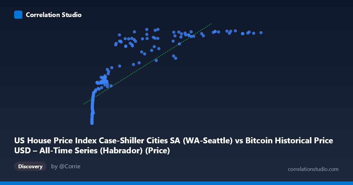
US House Price Index Case-Shiller Cities SA (WA-Seattle) vs Bitcoin Historical Price USD – All-Time Series (Habrador) (Price)
- Pearson correlation (r)
- 0.8155
- Spearman correlation
- 0.9673
- p-value
- 0
- Sample size (n)
- 187
- 95% confidence interval
- 0.761 to 0.8585
- Granger causality
- None
- Granger optimal lag
- 9
AI analysis
Analysis: Bitcoin Price vs. Seattle Case-Shiller Home Price Index
1. Relationship Overview
The scatterplot reveals a strong positive association between Bitcoin's historical USD price and the Seattle Case-Shiller Home Price Index, but the shape of this relationship is distinctly non-linear. At low Bitcoin values (under ~$1,000), the Seattle index climbs steeply from ~132 to ~220, while at high Bitcoin values (above ~$50,000), the index plateaus in the 370-400 range. This produces a classic logarithmic or saturating curve rather than a straight line — the data compresses heavily on the X-axis due to Bitcoin's exponential growth across its history, spanning nearly six orders of magnitude (0.06 to 118,670).
2. Strength, Direction, and Uncertainty
The linear Pearson correlation (r = 0.8155, R² = 0.665) indicates a strong positive relationship, with the linear model explaining about 66.5% of variance in Y. The 95% CI [0.761, 0.859] is fairly tight and excludes zero, and the p-value of 0 confirms this correlation is highly statistically significant — not a chance artifact. However, the note that Spearman's ρ exceeds Pearson's r is an important signal: the rank-order relationship is stronger than the linear one, confirming visually that a log/power transform of X would likely raise R² substantially beyond 0.665.
Critically, the Granger causality tests show no significant predictive direction in either direction (X→Y: p=0.532; Y→X: p=0.784). This means that despite the strong contemporaneous correlation, neither variable's past values help forecast the other's future values at the tested lag structure. This is a strong caveat: correlation here does not imply temporal leading/lagging causality — both series are likely driven by a shared external trend (time itself, or macroeconomic conditions) rather than one causing the other.
3. Notable Patterns and Outliers
The data clusters into two visually distinct regimes: a dense cluster of Bitcoin sub-$1,000 values paired with Seattle index values in the 130-220 range (reflecting Bitcoin's early years, 2010-2015), and a sparser cluster of Bitcoin values above $20,000 paired with index values in the 300-400 range (reflecting 2020-2025). There's relatively little data in the $1,000-$20,000 Bitcoin range, creating a visual gap. One mild inconsistency worth flagging: at X≈45,092 Y=313.10 and X≈29,111 Y=301.48 sit noticeably below the trend of neighboring points (e.g., X≈27,983 → Y=377.03), suggesting local volatility or a temporary Bitcoin crash/recovery misaligned with steadily rising home prices.
4. Confounding Factors and Caveats
The most significant confound is shared time trend: both Bitcoin price and Seattle home prices have risen dramatically over the 2010-2026 window due to broad macroeconomic forces (near-zero interest rates through the 2010s, pandemic-era stimulus, inflation, low housing supply, speculative capital inflows), not because one asset mechanically drives the other. This is a textbook case where two non-stationary time series trending upward will show spurious high correlation. The lack of Granger causality reinforces that this is likely a "common trend" artifact rather than genuine economic linkage. Additionally, Bitcoin's extreme scale/skew (mean 20,037 vs. median far lower) means the linear regression is disproportionately influenced by a handful of high-X points.
5. Recommendations for Further Investigation
First, refit using log(X) or log(X) vs log(Y) — given Spearman Pearson and the visibly saturating curve, a log-linear or power model should substantially improve fit and yield a more honest R². Second, to address the shared-trend confound, analysts should test correlation on de-trended or differenced series (e.g., month-over-month % changes in each) rather than raw levels — if the correlation collapses once trends are removed, it confirms this is spurious co-movement rather than a meaningful economic relationship. Third, given the Granger results, this pairing should not be used for predictive/trading purposes in its current form; instead, treat both as proxies for macro liquidity/risk appetite and consider a third common driver variable (e.g., M2 money supply, interest rates) that may explain both series more directly.
X dataset: Bitcoin Historical Price USD – All-Time Series (Habrador)
Y dataset: US House Price Index Case-Shiller Cities SA
Part of experiment: Bitcoin - Bitcoin Historical Price USD – All-Time Series (Habrador) vs US House Price Index Case-Shiller Cities SA