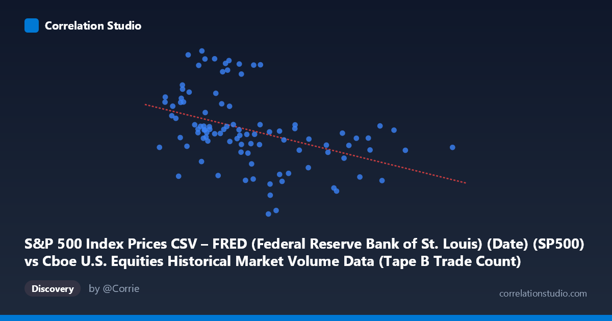
S&P 500 Index Prices CSV – FRED (Federal Reserve Bank of St. Louis) (Date) (SP500) vs Cboe U.S. Equities Historical Market Volume Data (Tape B Trade Count)
- Pearson correlation (r)
- -0.4197
- Spearman correlation
- -0.5121
- p-value
- 0.000017
- Sample size (n)
- 98
- 95% confidence interval
- -0.5706 to -0.2413
- Granger causality
- None
- Granger optimal lag
- 10
AI analysis
Analysis: S&P 500 Index Prices vs. Cboe Tape B Trade Count
Relationship Overview
The scatterplot reveals a moderate negative relationship between S&P 500 index prices and Cboe Tape B trade counts over the January–May 2026 period. As S&P 500 prices increase (moving rightward along the x-axis, ranging from ~657K to ~1.8M in index-scaled units), Tape B trade counts tend to decline. The linear regression equation (y = −0.000441804x + 7,386.13) quantifies this inverse slope, suggesting that higher equity valuations are associated with reduced trading activity specifically on Tape B securities — those listed on exchanges outside NYSE and Nasdaq (primarily regional exchange-listed equities). This directional finding is intuitive in broad strokes: rising markets can suppress certain speculative or reactive trading behaviors that concentrate in smaller-cap or regionally listed securities.
Correlation Strength, Significance, and Causality
The Pearson correlation of r = −0.4197 reflects a moderate negative association, but the explanatory power is modest — R² = 0.1761 means only 17.6% of the variance in Tape B trade counts is explained by S&P 500 price levels, leaving over 82% attributable to other factors. The 95% confidence interval for r spans [−0.5706, −0.2413], which is entirely negative and excludes zero, reinforcing that the negative direction is unlikely to be a sampling artifact. The p-value of 1.696 × 10⁻⁵ confirms the result is statistically significant at conventional thresholds (well below α = 0.01), and with N = 1,980 in the broader population and n = 98 paired samples, the sample is reasonably sized to support this inference. However, the Granger causality tests tell a meaningfully different story: neither direction (X→Y or Y→X) reaches significance at the optimal lag of 10 periods (F = 0.917, p = 0.523 and F = 1.052, p = 0.411, respectively). This means that while a contemporaneous correlation exists, S&P 500 prices do not temporally predict Tape B trade counts, nor vice versa — a critical caveat against any causal interpretation.
Patterns, Clusters, and Outliers
Several structural features are visible in the data. The bulk of observations cluster in the x-range of roughly 750K–1,150K, where Tape B trade counts span broadly from ~6,500 to ~7,500 — indicating high variability at moderate price levels, which dilutes the overall fit. At higher S&P values (1,300K), the data becomes sparser but trade counts are more consistently lower (roughly 6,500–6,950), tightening the scatter and reinforcing the negative trend at the upper range. Several notable outliers are visible: points near (1,085K, 6,344) and (1,115K, 6,369) represent unusually low Tape B counts at mid-range prices, potentially corresponding to low-volume trading days (holidays, half-days, or macro shock events). Conversely, points like (823K, 7,501) and (770K, 7,473) represent high trade counts at lower index values. There is also a suggestion of non-linearity: the negative trend appears steeper among lower-price observations and flattens somewhat at higher price levels, hinting that a logarithmic or piecewise model might better capture the relationship.
Confounding Factors and Interpretive Caveats
Several confounding factors warrant caution. First, day-of-week and holiday effects are well-documented drivers of equity trade counts, independent of price level. Second, market regime shifts within the January–May 2026 window — such as earnings seasons, Federal Reserve announcements, or geopolitical events — could simultaneously depress prices and elevate trading volume, creating spurious or amplified correlations. Third, the dataset metadata appears partially mismatched: the X-axis is labeled as S&P 500 prices but the values (~657K–1.8M) are orders of magnitude larger than typical S&P 500 index levels (~4,000–6,000), suggesting the X variable may actually represent a different metric (perhaps a total volume or notional value column mislabeled during dataset join). This discrepancy is a significant interpretive red flag that should be investigated before drawing firm conclusions. Finally, Tape B specifically covers NYSE American and regional exchange listings, which have distinct liquidity profiles that may respond differently to broad market conditions than the S&P 500 composite implies.
Actionable Insights and Further Investigation
Given these findings, several steps are recommended. First and most urgently, reconcile the X-axis scale discrepancy — if the variable truly represents S&P 500 prices, the units need verification; if it is another FRED series variable (e.g., total notional volume), the analysis framing should be updated accordingly. Second, incorporate additional control variables — VIX (volatility index), total market volume, and day-of-week indicators — into a multivariate regression to isolate the independent contribution of price levels to Tape B activity. Third, given the Granger non-causality result, analysts should avoid using one series to forecast the other in trading models without additional predictors. Fourth, testing a rolling correlation across the time window could reveal whether the r = −0.42 relationship is stable or driven by a specific sub-period, improving robustness. Finally, comparing Tape A and Tape C trade counts against the same X variable would contextualize whether this inverse relationship is specific to Tape B or a broader market-wide phenomenon.
X dataset: Cboe U.S. Equities Historical Market Volume Data
Y dataset: S&P 500 Index Prices CSV – FRED (Federal Reserve Bank of St. Louis) (Date)
Part of experiment: Daily - Cboe U.S. Equities Historical Market Volume Data vs S&P 500 Index Prices CSV – FRED (Federal Reserve Bank of St. Louis) (Date)