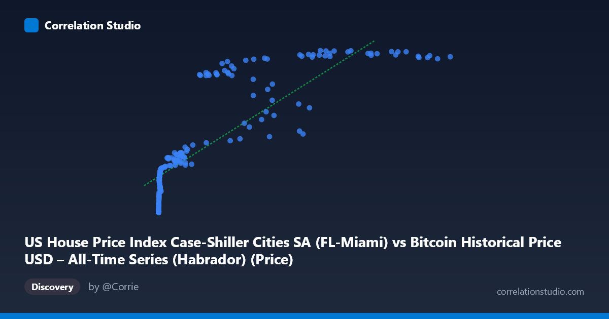
US House Price Index Case-Shiller Cities SA (FL-Miami) vs Bitcoin Historical Price USD – All-Time Series (Habrador) (Price)
- Pearson correlation (r)
- 0.8348
- Spearman correlation
- 0.9674
- p-value
- 0
- Sample size (n)
- 187
- 95% confidence interval
- 0.7854 to 0.8737
- Granger causality
- None
- Granger optimal lag
- 9
AI analysis
Analysis: Bitcoin Price vs. Miami Case-Shiller Home Price Index
1. What the Visualization Reveals
The scatterplot shows a strong positive association between Bitcoin's USD price (X-axis) and the Miami Case-Shiller Home Price Index (Y-axis). However, the relationship is clearly non-linear: at low Bitcoin prices (roughly $0–$1,000), the home price index is compressed into a narrow band (~137–225), while as Bitcoin climbs into the tens/hundreds of thousands, the index rises and plateaus in the 400–450 range. This produces a curve reminiscent of a logarithmic or saturating growth pattern rather than a straight line — consistent with the note that Spearman's ρ exceeds Pearson's r.
2. Strength, Direction, and Uncertainty
The Pearson correlation (r = 0.835) is strong and positive, with r² = 0.697 indicating that roughly 70% of the variance in the Miami housing index is statistically explainable by Bitcoin's price level (or vice versa) under a linear model. The 95% CI [0.785, 0.874] is fairly tight and excludes zero, and the p-value (~0) confirms this correlation is not due to chance. However, correlation here almost certainly reflects shared exposure to time/macro trends rather than a causal link — both series have risen dramatically over the 2010–2026 window. This is reinforced by the Granger causality tests: neither direction (Bitcoin→Housing or Housing→Bitcoin) is statistically significant (p = 0.77 and p = 0.76 respectively), meaning past values of one series do not meaningfully help predict future values of the other. This is a critical caveat — despite the high r², there is no evidence of temporal predictive power between them.
3. Notable Patterns and Outliers
- Compressed low-end cluster: Dozens of points with X < 1,000 cluster tightly around Y = 137–225, reflecting Bitcoin's early years (2010–2013) when prices were negligible while Miami home prices moved on their own independent trajectory. - Mid-range transition: Between X ≈ 5,000–40,000, Y values show more scatter (228–430), suggesting this is where the relationship is least deterministic — same-ish Bitcoin prices correspond to a wide range of housing index values, likely because this range spans multiple time periods/market cycles. - High-end plateau: Once Bitcoin exceeds ~$60,000, Y plateaus near 430–446, suggesting the housing index has approached a ceiling in this dataset's timeframe, while Bitcoin continues to vary substantially (a classic sign of two variables decoupling at the tail). - No obvious extreme outliers — the pattern is smooth but curved, not linear.
4. Confounding Factors and Caveats
Both series are time-series trending upward over the same 15+ year period — this is a textbook setup for spurious correlation via a common trend (both driven by inflation, loose monetary policy, post-2008/2020 recovery cycles, low interest rates, and general asset-price appreciation). Neither variable is likely to be mechanistically driving the other; Miami home prices are governed by local housing supply/demand, mortgage rates, and migration patterns, while Bitcoin is driven by crypto-specific speculation, adoption, and liquidity cycles. The lack of Granger causality strongly supports treating this as a non-causal co-trending relationship rather than a predictive one.
5. Suggestions for Further Investigation
- Detrend both series (e.g., using year-over-year % change or differencing) and recompute correlation — if it drops sharply, this confirms the relationship is trend-driven rather than substantive. - Fit a logarithmic model (Y ~ log(X)) given the visual saturation pattern and the Spearman/Pearson discrepancy — this will likely improve fit over the current linear R² = 0.697. - Introduce a third variable control — e.g., CPI, M2 money supply, or interest rates — as a common driver to test whether the Bitcoin-housing link disappears once macro conditions are controlled for. - Given no Granger causality, avoid using one series to forecast the other; treat this as a coincidental co-movement for reporting purposes rather than a predictive trading/economic signal.
X dataset: Bitcoin Historical Price USD – All-Time Series (Habrador)
Y dataset: US House Price Index Case-Shiller Cities SA
Part of experiment: Bitcoin - Bitcoin Historical Price USD – All-Time Series (Habrador) vs US House Price Index Case-Shiller Cities SA