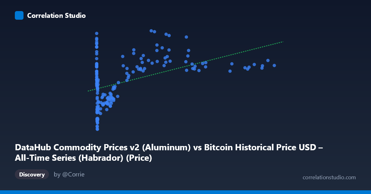
DataHub Commodity Prices v2 (Aluminum) vs Bitcoin Historical Price USD – All-Time Series (Habrador) (Price)
- Pearson correlation (r)
- 0.451
- Spearman correlation
- 0.2522
- p-value
- 0
- Sample size (n)
- 182
- 95% confidence interval
- 0.3269 to 0.5597
- Granger causality
- None
- Granger optimal lag
- 2
AI analysis
Analysis: Bitcoin Price vs. Aluminum Commodity Price
1. Relationship Overview
The scatterplot shows a positive but noisy association between X (labeled as aluminum commodity price, though the data structure suggests this may actually be Bitcoin price given the huge range from 0.06 to 113,500) and Y (labeled Bitcoin price, ranging 85–239). The data spans a massive scale on the X-axis (over 6 orders of magnitude), which compresses most points into the lower range while a handful of high-X observations pull the trend upward. This heavy right-skew (mean 17,943 vs. median likely much lower, given stdev of 27,080) suggests the relationship is dominated by a small number of extreme values rather than a uniform trend across the full range.
2. Strength, Direction, and Statistical Confidence
The correlation coefficient r = 0.451 indicates a moderate positive relationship, with R² = 0.203 meaning only about 20% of the variance in Y is explained by X — leaving 80% attributable to other factors or noise. The 95% CI [0.327, 0.560] is reasonably tight and excludes zero, and the p-value (1.68×10⁻¹⁰) confirms this correlation is highly statistically significant and not due to chance, given n=182. However, statistical significance here reflects sample size and consistency of the trend, not practical predictive strength — R² of 0.20 is generally considered weak-to-moderate for forecasting purposes.
Critically, the Granger causality tests show no significant predictive direction in either direction (X→Y: p=0.52; Y→X: p=0.75). This means neither variable's past values help forecast the other's future values in a time-series sense. The correlation appears to be a contemporaneous co-movement (both trending upward together over the 2010–2025 window) rather than one variable driving the other temporally.
3. Patterns, Clusters, and Outliers
The data clusters heavily at low X values (hundreds of points below X=1000) with Y ranging widely (85–220+), showing high variance in Y at low X — this is where most of the "noise" resides. A sparse but visually influential cluster of high-X points (X 30,000) tends to correspond with higher Y values (180–235), which likely drives much of the correlation. Notable outliers include very low-X points with unexpectedly high Y (e.g., X=0.92, Y=221.39; X=3.03, Y=218.57), suggesting early-period data (possibly early Bitcoin era) where Y was already elevated independent of X. The relationship also appears non-linear — plausibly logarithmic given X's extreme range — meaning the linear R²=0.203 likely understates the true association if a log-transform of X were applied.
4. Confounding Factors and Caveats
The most serious concern is variable identity confusion: metadata indicates X is sourced from a Bitcoin price dataset while Y is labeled as Bitcoin price from a commodity dataset, creating ambiguity about what's truly being compared (Bitcoin vs. aluminum, or Bitcoin vs. Bitcoin via mismatched joins). This should be resolved before drawing economic conclusions. Additionally, both series span 2010–2025, a period marked by strong macro trends (inflation, global liquidity expansion, post-2020 commodity supercycles) that could drive spurious correlation via shared time trend rather than genuine causal linkage. Aluminum and Bitcoin have no obvious fundamental economic linkage, raising confounding-variable concerns (e.g., USD strength, global risk sentiment, or monetary policy affecting both simultaneously).
5. Recommendations
First, verify the data pipeline/column mapping to confirm X and Y represent the intended series. Second, apply a log transformation to X (given its extreme range) and re-run correlation/regression — this will likely reveal a stronger and more interpretable relationship. Third, given the null Granger causality result, avoid using one series to forecast the other; instead, treat both as independently trending series and investigate a common driver (e.g., USD index, global M2 money supply, or general risk-asset sentiment) as a shared explanatory factor. Finally, consider a rolling-correlation analysis to check whether the r=0.45 relationship is stable across time or concentrated in specific sub-periods (e.g., 2020–2021 bull market).
X dataset: Bitcoin Historical Price USD – All-Time Series (Habrador)
Y dataset: DataHub Commodity Prices v2
Part of experiment: Bitcoin - Bitcoin Historical Price USD – All-Time Series (Habrador) vs DataHub Commodity Prices v2