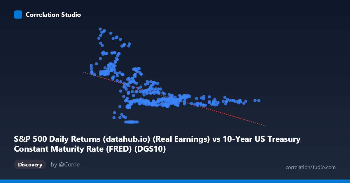
S&P 500 Daily Returns (datahub.io) (Real Earnings) vs 10-Year US Treasury Constant Maturity Rate (FRED) (DGS10)
- Pearson correlation (r)
- -0.5277
- Spearman correlation
- -0.4853
- p-value
- 0
- Sample size (n)
- 493
- 95% confidence interval
- -0.5886 to -0.4609
- Granger causality
- None
- Granger optimal lag
- 1
AI analysis
Analysis: S&P 500 Real Earnings vs. 10-Year Treasury Yield
1. Overall Relationship The scatterplot reveals a moderate negative relationship between the 10-Year US Treasury Constant Maturity Rate (X-axis) and S&P 500 Real Earnings (Y-axis), spanning data from 1962 to 2026. The linear regression equation (y = -7.635x + 115.932) indicates that for each one-percentage-point increase in the 10-year Treasury yield, real earnings are associated with a decline of approximately 7.6 units. Visually, this manifests as a downward-sloping trend, though with considerable scatter around the regression line, suggesting the relationship is real but far from deterministic.
2. Correlation Strength, Direction, and Causality The correlation coefficient of r = -0.528 indicates a moderate negative association. However, the R² of 0.278 is critical context: only about 27.8% of the variance in real earnings is explained by Treasury yields, meaning roughly 72% of variation stems from other sources. The 95% confidence interval of [-0.589, -0.461] is meaningfully narrow given N = 1,865, and the p-value of effectively zero confirms this is not a chance finding at any conventional significance threshold. That said, Granger causality tests find no significant predictive directionality in either direction (X→Y: F ≈ 0.000, p ≈ 0.999; Y→X: F = 0.373, p = 0.542). This is a crucial caveat — while the correlation is statistically robust, neither variable reliably predicts the other temporally at a one-period lag, suggesting the relationship may be driven by shared macro dynamics rather than a direct causal mechanism.
3. Notable Patterns, Clusters, and Outliers Several features stand out in the data. First, there is a dense cluster of observations between Treasury yields of 4–10% with real earnings between roughly 35–70, representing the bulk of modern economic experience. Second, there are striking high-earnings outliers at low yield levels — notably points such as (1.48, 202.44), (2.39, 207.57), (1.22, 217.26), and (3.26, 193.11) — which likely correspond to the post-2008 and COVID-era low-rate environments where earnings figures were volatile or distorted. Third, a small cluster of zero-value earnings observations (e.g., 4.18, 0.00 and 4.77, 0.00) may represent data anomalies, recession quarters, or reporting gaps that could distort the regression. The scatter also widens considerably at low X values, hinting at possible heteroscedasticity — the relationship becomes less predictable when yields are very low.
4. Confounding Factors and Caveats Several important caveats apply. The axis labels appear to be swapped or mislabeled in the metadata (X is described as "Real Earnings" from a Treasury dataset, and Y as "DGS10" from an S&P dataset), which warrants verification before drawing firm conclusions. Methodologically, this correlation spans over six decades during which the inflation regime, monetary policy framework, and earnings accounting standards changed substantially — pooling all periods together may obscure structurally distinct sub-regimes (e.g., the inflationary 1970s–80s vs. the low-rate post-GFC era). The zero-earnings outliers likely represent missing or censored data rather than true observations and could be inflating the apparent negative slope. Finally, omitted variables such as GDP growth, inflation expectations, profit margins, and equity risk premiums almost certainly co-determine both series.
5. Actionable Insights and Further Investigation Given these findings, several investigative steps are warranted. Segment the analysis by macroeconomic regime (e.g., pre-/post-1982 disinflation, post-2008 ZLB environment) to test whether the correlation is stable or regime-dependent — the outlier cluster at near-zero yields strongly suggests structural breaks. Remove or investigate the zero-earnings observations to assess their impact on the regression. Since Granger causality is absent at lag 1, test longer lags (4, 8, or 12 months) given that monetary policy transmission to corporate earnings typically operates over quarters to years. Additionally, controlling for inflation (CPI or PCE) would help isolate whether the yield–earnings link operates through real or nominal channels. Finally, consider a non-linear specification (e.g., piecewise linear or quadratic) given the apparent fanning of residuals at low yield values, which may better capture the true functional form of this historically important relationship.
X dataset: 10-Year US Treasury Constant Maturity Rate (FRED)
Y dataset: S&P 500 Daily Returns (datahub.io)
Part of experiment: Daily - 10-Year US Treasury Constant Maturity Rate (FRED) vs S&P 500 Daily Returns (datahub.io)