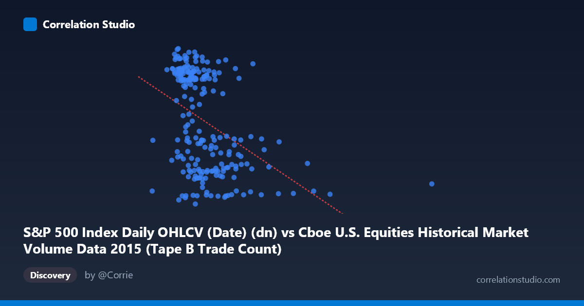
S&P 500 Index Daily OHLCV (Date) (dn) vs Cboe U.S. Equities Historical Market Volume Data 2015 (Tape B Trade Count)
- Pearson correlation (r)
- -0.4197
- Spearman correlation
- -0.4478
- p-value
- 0
- Sample size (n)
- 222
- 95% confidence interval
- -0.5225 to -0.3048
- Granger causality
- None
- Granger optimal lag
- 1
AI analysis
Analysis of S&P 500 Date Index vs. Cboe Tape B Trade Count (2015)
Relationship Overview The scatterplot reveals a negative relationship between the S&P 500 date index (a proxy for temporal progression through 2015) and the Cboe U.S. Equities Tape B Trade Count. As the date index increases across the February–December 2015 period, Tape B trade counts tend to decline. The linear regression equation (y = −3.35×10⁻⁵x + 125.76) confirms this downward trajectory, suggesting that Tape B trading activity systematically decreased over the course of 2015. Visually, the data points form a broad, dispersed cloud with a discernible downward tilt, consistent with a moderate but meaningful negative trend rather than a tight, deterministic relationship.
Correlation Strength and Statistical Significance The Pearson correlation of r = −0.42 indicates a moderate negative association, while r² = 0.176 means that only about 17.6% of the variance in Tape B trade counts is explained by the temporal progression captured by the date index — leaving roughly 82% attributable to other factors. The 95% confidence interval [−0.52, −0.30] is entirely negative, confirming consistent directionality, and the highly significant p-value (6.97×10⁻¹¹) rules out chance as an explanation. However, Granger causality tests find no significant predictive relationship in either direction (X→Y: F = 0.63, p = 0.43; Y→X: F = 0.46, p = 0.50), meaning that past values of the date index do not meaningfully predict future trade counts at the one-period lag tested, and vice versa. This combination — statistically significant correlation but no Granger causality — suggests the relationship reflects a shared temporal trend rather than a direct predictive or causal mechanism.
Notable Patterns, Clusters, and Outliers Several structural features stand out. The Y-axis data shows a bimodal-like spread, with trade counts clustering in two bands: a higher-activity zone (~120–127) and a lower-activity zone (~103–113), with relatively fewer observations in between. This banding may reflect distinct market regimes or seasonal patterns within 2015. There are also notable outliers on the X-axis: one point near X ≈ 1,014,195 (far right) and another near X ≈ 640,679 appear well separated from the main cluster (X range ~130,000–475,000), likely representing specific anomalous dates or data encoding irregularities. These extreme X-values with relatively low Y-values disproportionately anchor the regression slope and may be inflating the perceived strength of the negative correlation.
Confounding Factors and Caveats Several important caveats apply. First, the X-axis appears to encode dates as numeric values, meaning the "correlation" partly reflects the passage of time rather than a mechanistic link between S&P 500 behavior and Tape B volume. Second, market structure changes in 2015 — such as shifts in exchange fee schedules, regulatory changes, or competitive dynamics among trading venues — could independently drive Tape B trade count trends. Third, the two extreme outliers substantially influence the regression line; a robust regression excluding them might yield a weaker or differently shaped relationship. Finally, the column metadata appears cross-labeled (each dataset's column is attributed to the other), introducing uncertainty about whether the variables are precisely what they purport to be and warranting data provenance verification.
Actionable Insights and Further Investigation Given these findings, several next steps are warranted. Remove or flag the extreme outliers (X 600,000) and re-run the regression to assess their influence on r and slope estimates. Investigate the bimodal Y distribution by segmenting data into high- and low-activity regimes to determine whether separate correlations or distinct drivers exist within each cluster. Since Granger causality found no temporal predictive power at lag 1, test additional lags or apply rolling-window correlation analysis to detect non-stationary or regime-dependent relationships across the 2015 timeline. Finally, incorporate additional covariates — such as VIX (volatility index), overall market volume, and S&P 500 price levels — to build a multivariate model that can disentangle the temporal trend from genuine exchange-level trading dynamics.
X dataset: Cboe U.S. Equities Historical Market Volume Data 2015
Y dataset: S&P 500 Index Daily OHLCV (Date)
Part of experiment: Daily - Cboe U.S. Equities Historical Market Volume Data 2015 vs S&P 500 Index Daily OHLCV (Date)