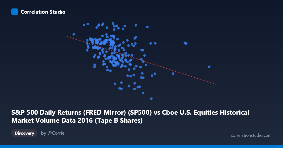
S&P 500 Daily Returns (FRED Mirror) (SP500) vs Cboe U.S. Equities Historical Market Volume Data 2016 (Tape B Shares)
- Pearson correlation (r)
- -0.4036
- Spearman correlation
- -0.4457
- p-value
- 0
- Sample size (n)
- 224
- 95% confidence interval
- -0.5078 to -0.2878
- Granger causality
- None
- Granger optimal lag
- 1
AI analysis
Scatterplot Analysis: S&P 500 Daily Returns vs. Cboe Tape B Shares (2016)
Relationship Overview
The scatterplot reveals a negative relationship between S&P 500 index levels (X-axis, proxying daily price via FRED mirror values) and Cboe Tape B share volume (Y-axis). As the S&P 500 value increases, Tape B share volume tends to decline modestly. The linear regression equation (y = -1.2427E-06x + 2244.33) confirms this downward slope, suggesting that higher equity valuations are associated with somewhat lower regional exchange share volume — a pattern consistent with the well-documented inverse relationship between market levels and trading activity, where calmer bull markets often see reduced urgency to trade.
Correlation Strength and Statistical Significance
The correlation coefficient of r = -0.4036 indicates a moderate negative association, but the explanatory power is limited: r² = 0.1629 means only ~16.3% of the variance in Tape B share volume is explained by S&P 500 levels, leaving over 83% attributable to other factors. The 95% confidence interval of [-0.5078, -0.2878] is entirely negative, providing reasonable statistical confidence that the relationship is genuinely inverse rather than a sampling artifact. The p-value of 3.47×10⁻¹⁰ confirms strong statistical significance given n = 224, so the direction of the relationship is reliable — but statistical significance should not be confused with practical magnitude, which remains modest. Critically, Granger causality testing found no significant predictive direction in either direction (X→Y: F = 0.33, p = 0.56; Y→X: F = 0.70, p = 0.40), meaning neither variable temporally predicts the other at a one-period lag. This effectively rules out a simple lead-lag trading signal between these two series.
Notable Patterns, Clusters, and Outliers
Several features stand out visually. The bulk of observations cluster in the X range of ~70M–140M with Tape B volumes between roughly 2,050–2,220, forming a moderately dense central cloud with substantial vertical scatter — reinforcing the weak-to-moderate fit. A handful of notable outliers deserve attention: the point near (201M, 2163) sits far to the right of the main cluster, representing an unusually high S&P 500 value day, yet its Tape B volume is unremarkable. Conversely, points with low Tape B volumes (~1,865–1,950) tend to cluster at mid-to-high X values (~110M–160M), consistent with the negative slope. The point at (43.5M, 2213) — the leftmost observation — represents the minimum X value with relatively high volume, consistent with the trend but extreme in X-space and potentially influential on the regression slope.
Confounding Factors and Caveats
Several important caveats apply. First, the dataset labels appear potentially swapped or misattributed: the X-axis is labeled as "S&P 500 Daily Returns" but the X values (43M–234M) clearly represent volume or notional figures, not price index levels (~1,865–2,272), which appear on the Y-axis labeled as "Tape B Shares." This metadata inconsistency warrants verification before drawing firm conclusions. Second, 2016 was an atypical year — it included Brexit volatility (June), the U.S. presidential election (November), and a Federal Reserve rate hike (December), all of which could create regime-dependent volume spikes that distort a single linear fit. Third, day-of-week effects, options expiration cycles, and index rebalancing events are known drivers of both volume and price behavior and are not controlled for here. Finally, with N = 2,609 population points but only n = 224 sampled, there is some risk of sample non-representativeness depending on the sampling scheme.
Actionable Insights and Further Investigation
Given the moderate correlation, limited explanatory power, and absent Granger causality, this relationship should not be used as a standalone trading or forecasting signal. Recommended next steps include: (1) verifying and correcting the axis/column label attribution to ensure the correct variables are being compared; (2) segmenting the data by market regime (pre/post-election, high/low VIX periods) to test whether the correlation is driven by specific episodes; (3) incorporating additional Cboe tape categories (Tape A, C) and total market volume to see if Tape B's relationship is idiosyncratic or systemic; (4) testing multivariate models that add volatility (VIX) as a covariate, since volatility independently drives both price moves and volume; and (5) examining the identified outliers (particularly the 201M and 43.5M X-value observations) to determine if they represent data errors or genuinely anomalous market days deserving separate treatment.
X dataset: Cboe U.S. Equities Historical Market Volume Data 2016
Y dataset: S&P 500 Daily Returns (FRED Mirror)
Part of experiment: Daily - Cboe U.S. Equities Historical Market Volume Data 2016 vs S&P 500 Daily Returns (FRED Mirror)