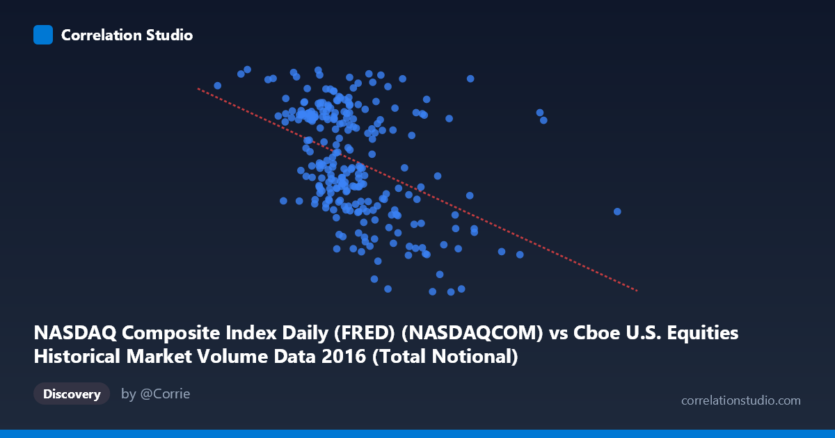
NASDAQ Composite Index Daily (FRED) (NASDAQCOM) vs Cboe U.S. Equities Historical Market Volume Data 2016 (Total Notional)
- Pearson correlation (r)
- -0.4337
- Spearman correlation
- -0.4522
- p-value
- 0
- Sample size (n)
- 252
- 95% confidence interval
- -0.5289 to -0.3277
- Granger causality
- None
- Granger optimal lag
- 10
AI analysis
Scatterplot Analysis: NASDAQ Composite Index vs. Cboe U.S. Equities Total Notional Volume (2016)
1. Overall Relationship The scatterplot reveals a moderate negative relationship between the NASDAQ Composite Index daily closing value and the total notional trading volume on Cboe U.S. equities markets during 2016. As the NASDAQ index rises, total notional volume tends to decline, and conversely, periods of lower index values are associated with higher trading volumes. This inverse pattern is visually apparent as a downward-sloping point cloud, though with considerable scatter around the trend line. The linear regression equation (y = −3.03×10⁻⁸x + 5563.07) confirms this negative slope, indicating that for every ~33 billion unit increase in notional volume, the NASDAQ index is expected to decrease by approximately 1 point.
2. Correlation Strength, Direction, and Statistical Context The Pearson correlation of r = −0.4337 indicates a moderate negative association. While statistically highly significant (p = 5.58×10⁻¹³, well below any conventional threshold), the R² of 0.1881 means that only ~18.8% of the variance in the NASDAQ index is explained by notional volume — leaving roughly 81% attributable to other factors. The 95% confidence interval of [−0.5289, −0.3277] is entirely negative and relatively narrow given the sample size (n = 252), reinforcing that the negative direction is reliable and not a sampling artifact. However, the Granger causality tests show no significant temporal predictive relationship in either direction (X→Y: F = 0.20, p = 0.996; Y→X: F = 0.57, p = 0.835), meaning that past notional volume does not help predict future NASDAQ levels, and past NASDAQ levels do not help predict future notional volume at the tested lag structure. This is a critical distinction: the correlation captures a contemporaneous association, not a lead-lag predictive one.
3. Notable Patterns, Clusters, and Outliers Several structural features stand out. The bulk of observations cluster in a core region of roughly X: 14–22 billion in notional volume and Y: 4,700–5,400 on the NASDAQ, forming a dense but diffuse cloud. There are notable right-tail outliers at very high notional volumes (25–41 billion), which tend to cluster at lower NASDAQ values (roughly 4,400–4,800), pulling the regression line and likely amplifying the negative correlation. One extreme point near X ≈ 41 billion appears as an isolated outlier far from the main cluster and warrants close inspection. A handful of points at low notional volume (X ≈ 7–13 billion) appear at middling NASDAQ values, suggesting some asymmetry. There is also a hint of heteroscedasticity — the spread in Y appears somewhat wider at moderate X values than at the extremes — which could modestly affect the precision of the linear fit.
4. Confounding Factors and Interpretive Caveats Several important caveats apply. First, 2016 was a year with distinct macro regimes — early-year volatility (January–February selloff), mid-year Brexit uncertainty, and a post-election rally in Q4 — each of which would simultaneously affect both index levels and trading volumes, creating spurious or regime-driven correlation rather than a structural relationship. High trading volume during selloffs naturally co-occurs with lower index values, which mechanically generates a negative correlation without implying any causal mechanism. Second, notional volume is itself partially a function of price level: when stock prices are higher, fewer shares may trade to generate equivalent notional value, creating a mathematical coupling between the two variables. Third, the axes appear to be swapped in the dataset metadata (the NASDAQ index is listed under "Total Notional" and vice versa), which, if reflecting an actual data preparation inconsistency, would require verification before drawing firm conclusions. Finally, daily data introduces autocorrelation in both series, which can inflate the apparent significance of the correlation if not properly accounted for.
5. Actionable Insights and Further Investigation Given the moderate but unexplained majority of variance, several next steps would strengthen interpretation. Regime segmentation — splitting the data into pre- and post-Brexit, pre- and post-election quarters — would reveal whether the negative correlation is consistent or driven by specific volatility episodes. Investigating the high-volume outlier days individually (e.g., January 2016 selloff, November 2016 election) could clarify whether those extreme points are structurally informative or noise-amplifying anomalies. Since Granger causality found no predictive direction at a 10-period lag, testing shorter lags (1–3 days) may be worthwhile, as intraday volume-price dynamics in equities typically operate at much shorter horizons. Additionally, controlling for the VIX (volatility index) as a covariate in a multiple regression framework would help disentangle whether the volume-index relationship is direct or mediated entirely through market stress. Finally, extending the analysis to multiple years would test whether this negative relationship is a stable structural feature of NASDAQ-listed equity markets or an artifact of 2016's unique macro environment.
X dataset: Cboe U.S. Equities Historical Market Volume Data 2016
Y dataset: NASDAQ Composite Index Daily (FRED)
Part of experiment: Daily - Cboe U.S. Equities Historical Market Volume Data 2016 vs NASDAQ Composite Index Daily (FRED)