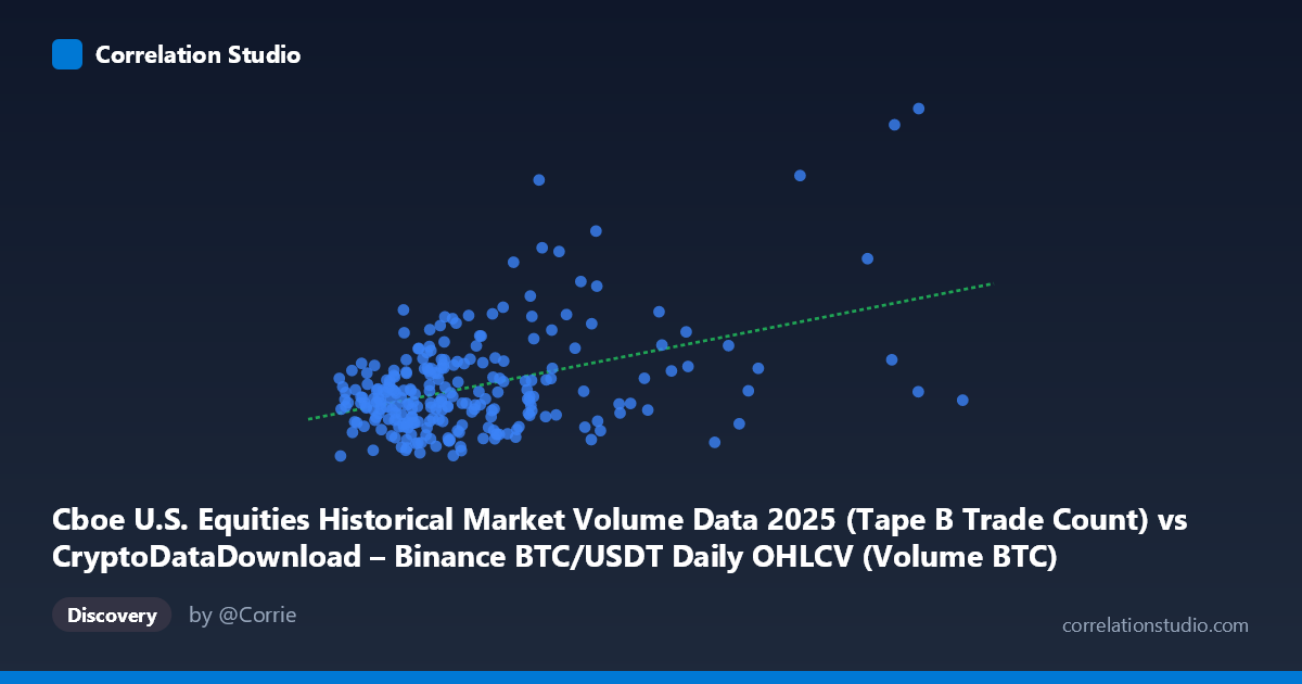
Cboe U.S. Equities Historical Market Volume Data 2025 (Tape B Trade Count) vs CryptoDataDownload – Binance BTC/USDT Daily OHLCV (Volume BTC)
- Pearson correlation (r)
- 0.4288
- Spearman correlation
- 0.2331
- p-value
- 0
- Sample size (n)
- 250
- 95% confidence interval
- 0.3219 to 0.525
- Granger causality
- None
- Granger optimal lag
- 10
- Time coverage
- 2025-01-02 to 2025-12-31
AI analysis
Analysis: Cboe Trade Count vs. Binance BTC/USDT Volume
1. Relationship Overview
The scatterplot depicts a modest positive association between two variables that, on their face, come from entirely different markets: X represents Cboe U.S. equities trade counts (Tape B), while Y represents Binance BTC/USDT trading volume. The data cloud shows a general upward drift — as X increases, Y tends to increase — but with substantial scatter around any fitted line. Most points cluster in the lower-X range (roughly 10,000–25,000), with a sparser tail extending to higher X values (up to ~83,600), giving the visualization a somewhat heteroscedastic, fan-shaped appearance.
2. Strength, Direction, and Statistical Confidence
The correlation coefficient (r = 0.429) indicates a weak-to-moderate positive linear relationship. Critically, r² = 0.184 means only 18.4% of the variance in Y is explained by X — the remaining ~82% is driven by other factors entirely. The 95% CI [0.322, 0.525] is reasonably tight and excludes zero, and the p-value (1.32E-12) confirms this correlation is highly statistically significant — but statistical significance here reflects the large sample size more than practical predictive power. A significant-but-weak r is common with n=250; it tells us the relationship is real but not strong enough to rely on for prediction. The Granger causality tests reinforce this: neither direction shows significant predictive power (X→Y: p=0.61; Y→X: p=0.57), meaning neither series' past values help forecast the other's future values at the tested lag structure. This strongly suggests the correlation is contemporaneous/coincidental rather than causal or lead-lagging.
3. Notable Patterns and Outliers
Several points stand out: a cluster around X≈32,000–42,000 with Y values exceeding 1,000,000 (e.g., 37,920 → 1,065,771; 39,835 → 1,048,393) appears to pull the regression slope upward — these may be influential high-leverage points given the sparse density at higher X. Conversely, some low-to-mid X points also reach high Y values (e.g., 22,557 → 925,641; 19,834 → 884,029), suggesting Y has considerable independent variability unrelated to X. The bulk of low-Y outcomes (400,000–600,000) span nearly the entire X range, indicating X alone poorly discriminates Y's level. No clear non-linear curvature (log, exponential) is obvious; the scatter looks like linear-with-heavy-noise rather than a curved relationship.
4. Confounding Factors and Caveats
This pairing is econometrically unusual — comparing equity market microstructure (Tape B trade counts) to crypto trading volume lacks an obvious economic mechanism. Any correlation is more plausibly explained by shared confounders such as: - Common temporal trends: both markets may exhibit rising activity over 2025 due to macro conditions, volatility regimes, or seasonal effects, creating spurious correlation via time-trend alignment rather than genuine interaction. - Volatility clustering: high-volatility days often see elevated volume/trade-count across all markets simultaneously (risk-on/risk-off dynamics), inflating cross-asset correlation without causality. - Data alignment issues (time zones, trading-day mismatches between 24/7 crypto and equity market hours) could introduce noise or spurious alignment.
5. Recommendations
Given the weak r², non-significant Granger results, and lack of causal mechanism, this correlation should not be used for cross-market predictive trading strategies. Instead: (1) test both series for common trends/unit roots and consider detrending or first-differencing before re-assessing correlation, to rule out spurious trend-driven association; (2) investigate whether a third variable (e.g., overall market volatility index, day-of-week effects, or macro news events) explains co-movement in both; (3) examine the high-Y outlier cluster (X 32k–42k) for specific date matches — these could reflect notable market events (e.g., late 2025 volatility spikes) worth case-study investigation rather than treating as part of a stable linear relationship.
X dataset: CryptoDataDownload – Binance BTC/USDT Daily OHLCV
Y dataset: Cboe U.S. Equities Historical Market Volume Data 2025
Part of experiment: Bitcoin - CryptoDataDownload – Binance BTC/USDT Daily OHLCV vs Cboe U.S. Equities Historical Market Volume Data 2025