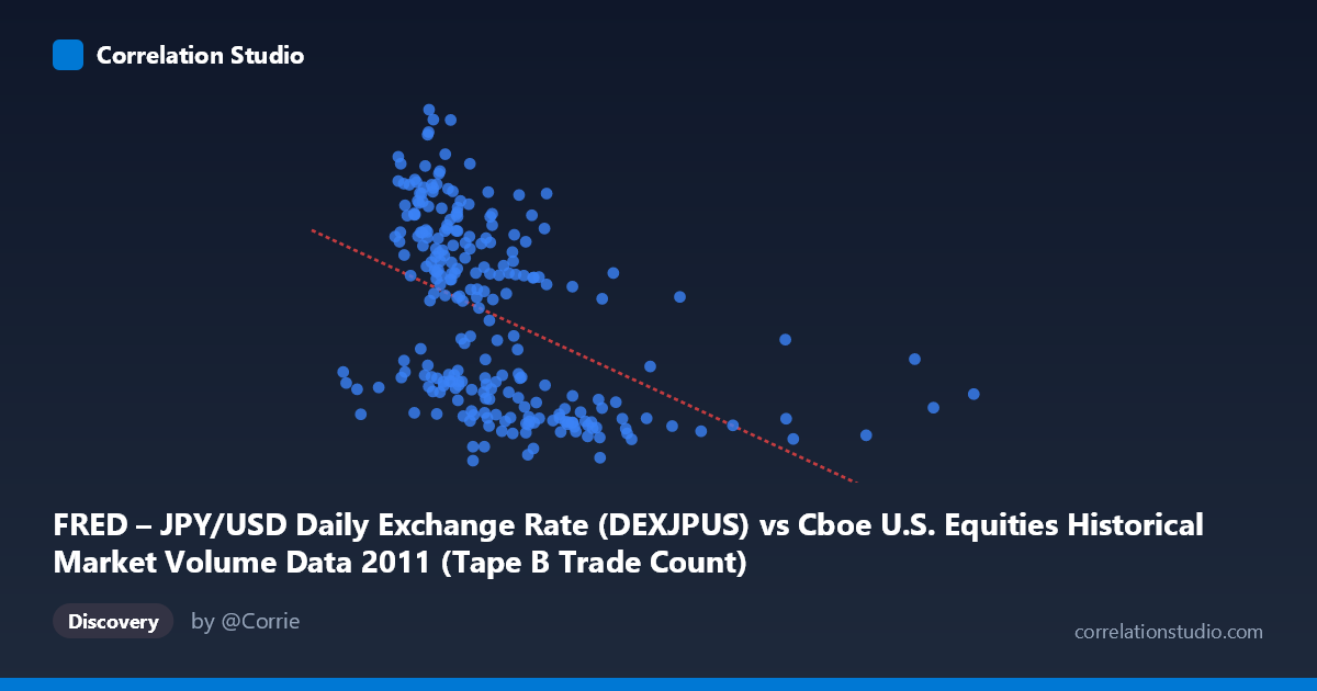
FRED – JPY/USD Daily Exchange Rate (DEXJPUS) vs Cboe U.S. Equities Historical Market Volume Data 2011 (Tape B Trade Count)
- Pearson correlation (r)
- -0.4632
- Spearman correlation
- -0.5928
- p-value
- 0
- Sample size (n)
- 250
- 95% confidence interval
- -0.5553 to -0.3598
- Granger causality
- None
- Granger optimal lag
- 1
AI analysis
Analysis of JPY/USD Exchange Rate vs. Cboe Tape B Trade Count (2011)
1. What the Visualization Reveals
The scatterplot displays a moderate negative relationship between U.S. equity market trading volume (Tape B trade count, on the X-axis) and the JPY/USD daily exchange rate (on the Y-axis) across 2011. As trade counts increase, the yen tends to appreciate against the dollar (i.e., fewer yen per dollar, meaning a stronger yen). The data are notably heteroscedastic — at lower trade count values (roughly 150,000–350,000), Y values are widely dispersed across the full range of ~75–85, while at higher trade counts the Y values compress toward the lower end of the range (77–80), suggesting that high-volume trading days are almost exclusively associated with a stronger yen.
2. Correlation Strength, Direction, and Causality
The Pearson r of -0.463 indicates a moderate negative correlation, but the r² of 0.2145 is the more sobering statistic — only 21.5% of the variance in the JPY/USD rate is explained by Tape B trade count. The remaining ~78.5% is driven by factors entirely outside this model. The 95% confidence interval of [-0.555, -0.360] is reasonably tight and does not cross zero, and the p-value of 1.07×10⁻¹⁴ confirms the relationship is highly statistically significant given the sample size of 250 (drawn from N=3,780). However, statistical significance here is partly a function of sample size and should not be confused with practical importance. Critically, Granger causality tests find no significant predictive direction in either direction (X→Y: p=0.825; Y→X: p=0.614), meaning that knowing yesterday's trade count does not help predict today's exchange rate, and vice versa. This rules out simple temporal lead-lag exploitation of this relationship for trading or forecasting purposes.
3. Notable Patterns, Clusters, and Outliers
Several structural features stand out. There is a visible right-skewed cluster of high-volume outliers — notably points near 616,000, 617,000, and 832,000 trade counts — all congregating in the 76.5–79.5 Y range, which is consistent with the heteroscedasticity described above. A point at approximately (207,845; 85.26) stands out as a potential high-leverage outlier, representing both a low trade count day and the highest yen-per-dollar value in the dataset (weakest yen). The hint from the Spearman ρ exceeding Pearson r also suggests the true relationship may be non-linear — likely logarithmic or monotonic but curved — meaning the linear regression line (y = -1.10×10⁻⁵x + 82.79) likely underestimates the steepness of the relationship at low trade counts and overestimates it at high counts. A logarithmic or polynomial fit would likely improve explanatory power meaningfully.
4. Confounding Factors and Interpretive Caveats
The most significant caveat is the axis assignment anomaly: the dataset labels suggest the X-axis is from the JPY/USD FRED dataset while the Y-axis is from the Cboe volume dataset — this appears inverted from the column names described, and care should be taken to confirm which variable is truly being treated as the potential predictor. Beyond this, 2011 was an extraordinary year for both variables — it included the Tōhoku earthquake/tsunami (March 2011), which caused dramatic yen appreciation and likely spiked equity trading volumes simultaneously, potentially manufacturing a spurious correlation driven by a single macro shock. Both variables are also susceptible to common drivers such as global risk sentiment (VIX), Federal Reserve policy signals, and U.S. equity market volatility, any of which could be the true underlying cause of co-movement. The cross-dataset pairing of a currency rate with a market microstructure metric is inherently fragile without controlling for these macro factors.
5. Actionable Insights and Further Investigation
Given the non-causality finding and modest r², this correlation is not suitable as a standalone predictive signal, but it may be a useful component in a multivariate model. Recommended next steps include: (1) fitting a logarithmic regression to test whether the Spearman-Pearson divergence is resolved and r² improves; (2) segmenting the data temporally to test whether the correlation is driven disproportionately by the March 2011 shock period versus the rest of the year; (3) adding VIX or S&P 500 volatility as a control variable to test whether the observed correlation is merely a proxy for risk-off episodes; and (4) extending to multi-year data to determine whether this relationship is stable across years or specific to 2011's unique macro environment. If the relationship persists after controlling for volatility regime, it could inform currency-hedging strategies for equity market makers with JPY exposure.
X dataset: Cboe U.S. Equities Historical Market Volume Data 2011
Y dataset: FRED – JPY/USD Daily Exchange Rate
Part of experiment: Daily - Cboe U.S. Equities Historical Market Volume Data 2011 vs FRED – JPY/USD Daily Exchange Rate