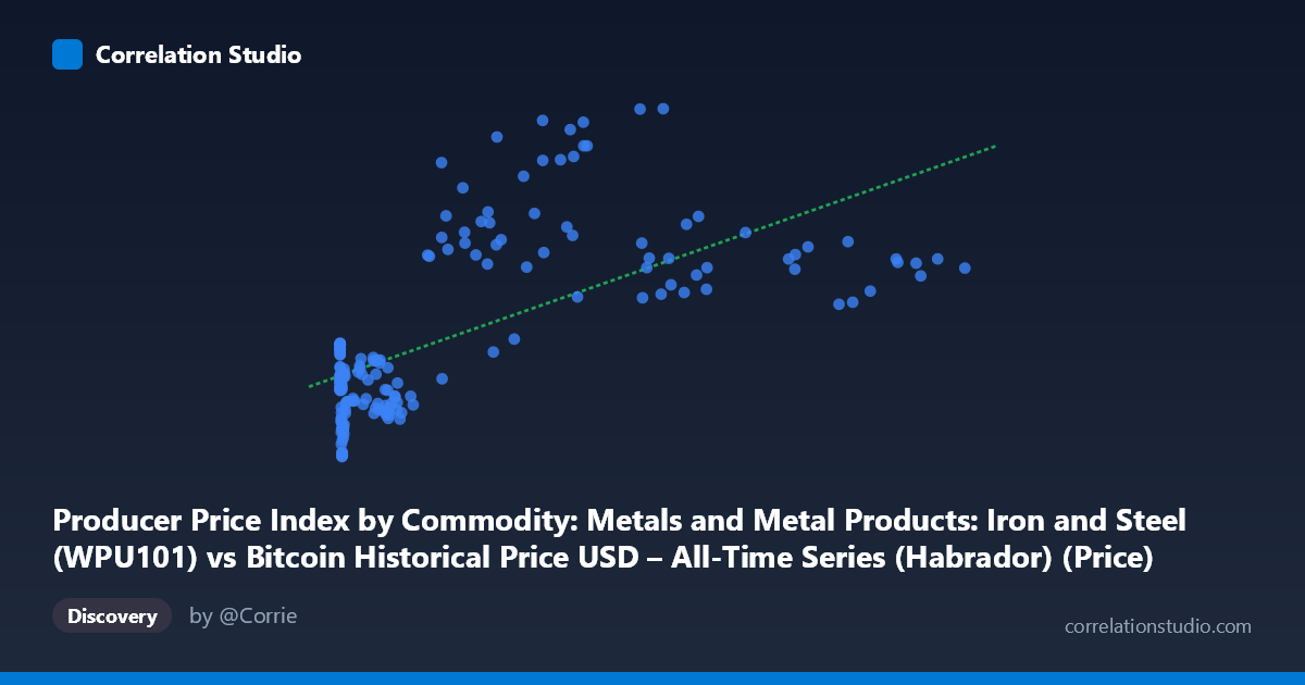
Producer Price Index by Commodity: Metals and Metal Products: Iron and Steel (WPU101) vs Bitcoin Historical Price USD – All-Time Series (Habrador) (Price)
- Pearson correlation (r)
- 0.657
- Spearman correlation
- 0.5572
- p-value
- 0
- Sample size (n)
- 189
- 95% confidence interval
- 0.5674 to 0.7311
- Granger causality
- None
- Granger optimal lag
- 2
AI analysis
Analysis: Bitcoin Price vs. Iron and Steel PPI
1. What the Visualization Reveals
The scatterplot shows a positive but noticeably non-linear relationship between Bitcoin's historical USD price (X-axis) and the Producer Price Index for Iron and Steel (Y-axis). At low Bitcoin price levels (under ~$1,000), the PPI values cluster tightly in the 170–260 range with considerable scatter, reflecting the early years of Bitcoin's history (2010–2013) when steel prices moved independently through their own economic cycles. As Bitcoin's price climbs into the tens of thousands, PPI values shift upward into the 280–430 range, but the relationship becomes less about Bitcoin driving steel prices and more about both series trending upward over the same 2010–2026 macroeconomic period.
2. Strength, Direction, and Uncertainty
The correlation coefficient (r = 0.657) indicates a moderate-to-strong positive linear relationship, with r² = 0.432 meaning only about 43% of the variance in steel PPI is statistically explained by Bitcoin price—leaving more than half unexplained. The 95% confidence interval [0.567, 0.731] is reasonably tight and does not cross zero, and the p-value of ~0 confirms this correlation is highly unlikely to be due to chance given the sample. However, statistical significance of correlation should not be conflated with causal or predictive power: the Granger causality tests show no significant predictive direction in either direction (Bitcoin→PPI: p=0.121; PPI→Bitcoin: p=0.547). This is a critical distinction—the two series are correlated in level but neither reliably "leads" or forecasts the other over time, suggesting the relationship is likely driven by a shared external trend (e.g., broad inflation, dollar devaluation, or global monetary expansion) rather than any direct economic linkage between crypto markets and steel manufacturing.
3. Notable Patterns and Outliers
The data displays a clear log-linear or threshold-like structure rather than pure linearity: PPI values stay flat and compressed while Bitcoin trades under $1,000, then increase more variably as Bitcoin scales into the thousands and tens of thousands. Several notable outliers exist—points like (56973.18, 433.25) and (44354.64, 397.64) show unusually high PPI relative to neighboring Bitcoin prices (e.g., 41869.55→395.23 vs. 45092.81→292.20), suggesting steel price spikes (likely tied to 2021–2022 supply chain disruptions and inflation surges) that coincided with, but weren't necessarily caused by, Bitcoin's price level at the time. The extreme range of X (0.06 to 118,670) compressed on a linear scale likely causes visual crowding near the origin, masking finer structure in Bitcoin's low-price era.
4. Confounding Factors and Caveats
The most significant caveat is that both variables are essentially time-indexed series, not independently sampled observations—Bitcoin's price has a well-known multi-year secular uptrend, and steel PPI has its own inflation-driven upward trajectory, especially post-2020. Any two upward-trending time series will show spurious correlation regardless of true causal linkage; this is a classic case where correlating non-stationary time series can inflate r without meaningful economic relationship. Macroeconomic confounders—USD inflation, global supply chain conditions, interest rates, and general risk-asset sentiment—likely drive both series simultaneously. Additionally, the sample (n=189) is unevenly distributed across time (dense in some price ranges, sparse in others), which can bias regression estimates.
5. Actionable Insights
Given the lack of Granger causality, this correlation should not be used for predictive or trading purposes in either direction. Analysts should test for cointegration or run the correlation on detrended/differenced series (e.g., % monthly changes) rather than raw levels, which would better isolate whether short-term co-movements exist beyond the shared trend. It would also be valuable to control for a common macro variable (e.g., CPI or M2 money supply) via partial correlation to determine whether the Bitcoin-PPI relationship disappears once broader inflation is accounted for—which seems the most plausible underlying driver of this pattern.
X dataset: Bitcoin Historical Price USD – All-Time Series (Habrador)
Y dataset: Producer Price Index by Commodity: Metals and Metal Products: Iron and Steel
Part of experiment: Bitcoin - Bitcoin Historical Price USD – All-Time Series (Habrador) vs Producer Price Index by Commodity: Metals and Metal Products: Iron and Steel