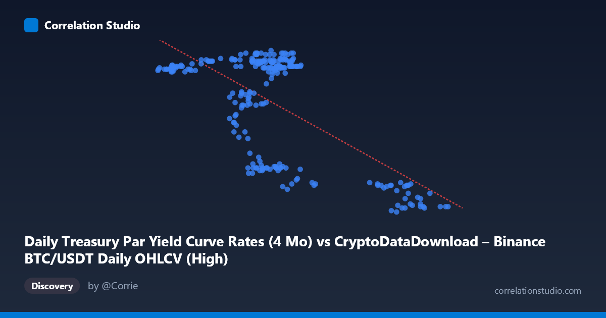
Daily Treasury Par Yield Curve Rates (4 Mo) vs CryptoDataDownload – Binance BTC/USDT Daily OHLCV (High)
- Pearson correlation (r)
- -0.6587
- Spearman correlation
- -0.3331
- p-value
- 0
- Sample size (n)
- 250
- 95% confidence interval
- -0.7237 to -0.5823
- Granger causality
- None
- Granger optimal lag
- 1
AI analysis
Analysis: Treasury Par Yield (4 Mo) vs. BTC/USDT Daily High
(Note: axis labels appear swapped in the metadata — the data itself shows X spanning ~40,000–108,000 and Y spanning ~4.3–5.5, so X is behaving as the BTC price series and Y as the yield series. The analysis below follows the actual numeric behavior in the data.)
1. What the Visualization Reveals The scatterplot shows a clear downward-sloping relationship: as X increases, Y systematically decreases. Points cluster tightly in two regions — a dense cluster where X is roughly 43,000–72,000 and Y sits high (5.1–5.5), and a sparser cluster where X exceeds 90,000 and Y drops to 4.3–4.6. This bimodal clustering, rather than a smooth continuous decline, suggests two distinct regimes rather than a single uniform linear process.
2. Strength, Direction, and Statistical Confidence The correlation coefficient (r = -0.6587) indicates a moderately strong negative relationship, with r² = 0.434 meaning only about 43% of the variance in Y is explained by X — leaving the majority (57%) driven by other factors. The 95% CI [-0.724, -0.582] is reasonably tight and entirely negative, and the p-value of ~0 confirms this relationship is highly unlikely to be due to chance at this sample size (n=250). However, statistical significance here reflects sample size and consistency of direction, not necessarily strength of practical predictive power — r² of 0.43 still leaves substantial unexplained variance. Critically, the Granger causality tests show no significant predictive direction in either direction (X→Y: p=0.44; Y→X: p=0.36), indicating that despite the strong contemporaneous correlation, neither series reliably predicts future movements of the other at a 1-period lag. This is an important distinction: correlation without Granger causality suggests the relationship may be driven by a shared external factor or simply a static/contemporaneous association rather than a lead-lag dynamic.
3. Notable Patterns and Outliers The data is not uniformly distributed along the regression line — it shows clear clustering rather than a continuous spread, consistent with two "regimes": a high-X/low-Y regime (X 90,000, Y ≈ 4.3–4.5) and a low/mid-X/high-Y regime (X 43,000–72,000, Y ≈ 5.1–5.5). Within the dense lower-X cluster there is also a secondary sub-pattern: several points near X=60,000–70,000 have notably lower Y values (4.5–4.9) mixed among high-Y points, suggesting some non-linearity or an additional variable creating scatter within that regime. This clustering pattern, rather than a smooth linear decay, hints that the relationship might be better modeled as a threshold or regime-switching effect rather than a strictly linear one, even though the linear fit captures a moderate share of variance.
4. Confounding Factors and Caveats Both series are time-based (2024 full-year daily data), so this is likely a case of spurious or indirect correlation driven by a shared macro trend over time — e.g., both BTC price levels and short-term Treasury yields could be independently influenced by Federal Reserve policy shifts, inflation expectations, or macro liquidity conditions throughout 2024, without one directly causing the other. Since both series are non-stationary trending time series, the Pearson correlation can be inflated by shared trend components (a classic time-series pitfall) — this may explain the strong r despite the absence of Granger causality. Additionally, daily financial data often carries autocorrelation (today's value is close to yesterday's), which violates the independence assumption underlying standard significance tests and can artificially shrink p-values.
5. Actionable Insights and Further Investigation Given the lack of Granger causality, this relationship should not be used for short-term predictive trading or rate-forecasting models based on lagged values. Instead, analysts should: (1) test both series for stationarity (e.g., ADF test) and consider differencing or detrending before re-estimating correlation, to check whether the relationship survives when shared trend is removed; (2) investigate common macro drivers (Fed rate decisions, CPI releases, risk-on/risk-off sentiment) that could jointly explain both series' movements; (3) explore the apparent two-regime clustering with a structural break test or regime-switching model rather than a single linear fit; and (4) extend the lag window in Granger tests (beyond 1 period) to check for longer-horizon lead-lag effects, since monetary policy impacts on risk assets often materialize over weeks rather than a single day.
X dataset: CryptoDataDownload – Binance BTC/USDT Daily OHLCV
Y dataset: Daily Treasury Par Yield Curve Rates
Part of experiment: Bitcoin - CryptoDataDownload – Binance BTC/USDT Daily OHLCV vs Daily Treasury Par Yield Curve Rates