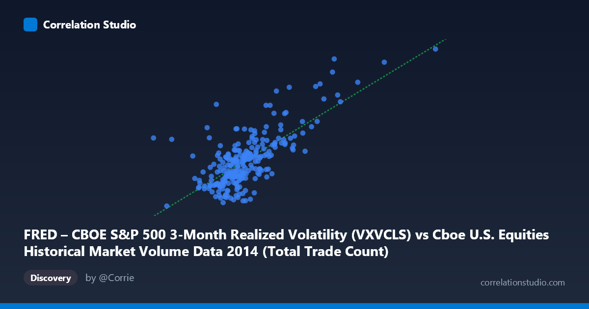
FRED – CBOE S&P 500 3-Month Realized Volatility (VXVCLS) vs Cboe U.S. Equities Historical Market Volume Data 2014 (Total Trade Count)
- Pearson correlation (r)
- 0.7239
- Spearman correlation
- 0.619
- p-value
- 0
- Sample size (n)
- 252
- 95% confidence interval
- 0.6593 to 0.7779
- Granger causality
- X → Y
- Granger optimal lag
- 1
AI analysis
Analysis: CBOE S&P 500 3-Month Realized Volatility vs. Total Trade Count (2014)
Relationship Overview The scatterplot reveals a moderately strong positive relationship between CBOE S&P 500 3-Month Realized Volatility (VXVCLS) and Total Trade Count in U.S. equities markets across 2014. As realized volatility increases, total trade count tends to rise commensurately, which aligns intuitively with market microstructure theory: elevated volatility environments typically drive heightened trading activity as market participants reposition, hedge, and respond to price uncertainty. The linear regression equation (y = 3.62×10⁻⁶x + 8.147) confirms a positive slope, though the relatively small coefficient suggests the relationship, while directionally clear, involves substantial scale differences between the two variables.
Correlation Strength and Statistical Significance The Pearson correlation of r = 0.724 indicates a meaningful positive association, with r² = 0.524 meaning that approximately 52.4% of the variance in volatility is explained by trade count — a substantial but incomplete picture, leaving nearly half the variance attributable to other factors. The 95% confidence interval of [0.659, 0.778] is reassuringly narrow given the sample size of n = 252, and the p-value of effectively zero confirms this relationship is not a statistical artifact. Critically, the Granger causality analysis establishes a unidirectional temporal predictive relationship: trade count (X) Granger-causes volatility (Y) at a 1-period lag (F = 4.621, p = 0.033), while the reverse direction is statistically insignificant (F = 0.371, p = 0.543). This suggests that elevated market trading volume today carries predictive information about volatility tomorrow, which has meaningful practical implications for risk monitoring and early-warning systems.
Notable Patterns, Clusters, and Outliers The sample points reveal a relatively tight central cluster between trade counts of roughly 1.6M–2.3M paired with volatility readings of 13–17, suggesting this represents the dominant "normal market" regime for 2014. However, several notable outliers are visible at the upper right — points such as (3,772,957; 22.85), (3,153,910; 23.09), and (2,766,118; 17.62) — representing episodes of simultaneously extreme volume and volatility, likely corresponding to identifiable market stress events in 2014 (e.g., geopolitical tensions, Fed communications, or the October 2014 equity selloff). There is also a modest lower-left cluster around trade counts near 920K–1.5M with moderate volatility readings, potentially reflecting holiday-shortened sessions or low-liquidity periods. The spread widens noticeably at higher trade counts, suggesting mild heteroscedasticity — variance in volatility increases as volume rises — which warrants caution when applying the linear model at extremes.
Confounding Factors and Caveats Several important caveats temper interpretation. First, Granger causality is not true causality: the finding that trade count predicts volatility may reflect a common underlying driver (e.g., macroeconomic news releases simultaneously boost both volume and uncertainty) rather than a direct mechanistic link. Second, the 3-month realized volatility metric is by construction a backward-looking, smoothed measure, which may artificially inflate correlation with contemporaneous volume by embedding prior high-volume days within the calculation window. Third, 2014 was a relatively contained volatility regime (mean VXV ≈ 15.6), and the relationship observed here may not generalize to crisis periods where the dynamic between volume and volatility can become non-linear or even inverted (e.g., liquidity withdrawal during flash crashes). Finally, the population of N = 3,686 underlying data points versus the n = 252 sample should prompt verification that the sampling strategy captures the full distribution of market conditions without selection bias.
Actionable Insights and Further Investigation The unidirectional Granger causality result is the most actionable finding here: monitoring daily trade count could serve as a leading indicator for next-day volatility regime shifts, which is directly useful for options pricing desks, risk managers calibrating VaR models, and algorithmic traders adjusting position sizing. Practically, a threshold-based alert system — flagging days when trade count exceeds, say, 2.5M — could serve as an early signal for elevated volatility regimes. For further investigation, it would be valuable to: (1) test non-linear models (e.g., log-log regression or spline fits) given the apparent heteroscedasticity; (2) extend the time series beyond 2014 to test whether the Granger relationship holds across different volatility regimes; (3) decompose trade count by exchange or trade type (lit vs. dark pool) to identify which component most strongly drives the predictive relationship; and (4) control for macro event calendars (FOMC dates, earnings seasons) to isolate whether the correlation persists after accounting for shared news-driven spikes.
X dataset: Cboe U.S. Equities Historical Market Volume Data 2014
Y dataset: FRED – CBOE S&P 500 3-Month Realized Volatility
Part of experiment: Daily - Cboe U.S. Equities Historical Market Volume Data 2014 vs FRED – CBOE S&P 500 3-Month Realized Volatility