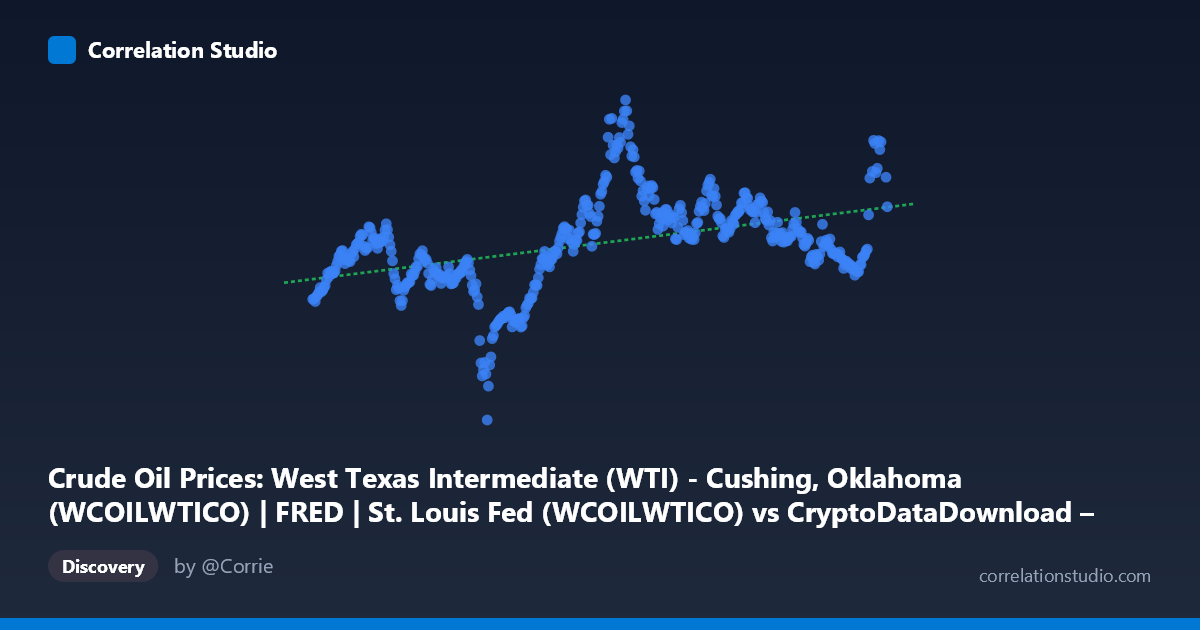
Crude Oil Prices: West Texas Intermediate (WTI) - Cushing, Oklahoma (WCOILWTICO) | FRED | St. Louis Fed (WCOILWTICO) vs CryptoDataDownload – Binance BTC/USDT Daily OHLCV (Unix)
- Pearson correlation (r)
- 0.4362
- Spearman correlation
- 0.5
- p-value
- 0
- Sample size (n)
- 458
- 95% confidence interval
- 0.3589 to 0.5075
- Granger causality
- None
- Granger optimal lag
- 1
- Time coverage
- 2017-08-18 to 2026-06-19
- Recomputed on refreshed data
- 2026-10-08 (r was 0.4362)
AI analysis
Analysis: WTI Crude Oil Prices vs. Time (Mislabeled Axes)
Important note on data labeling: The axis labels appear swapped or mismatched in the metadata—X is described as a timestamp column but the data shows X values as Unix timestamps (dates from 2017-2026) while Y values (3.32–120.43) are clearly WTI crude oil prices in USD/barrel. This analysis proceeds treating X as time and Y as WTI oil price, which matches the actual data structure.
1. What the Visualization Shows The scatterplot tracks WTI crude oil prices over roughly nine years (August 2017 to June 2026). Prices range widely from $3.32 (likely the historic negative-adjacent crash period of April 2020) to $120.43, with a mean of $67.92 and substantial volatility (stdev ~$17.31). The data shows clear cyclical behavior rather than a simple linear trend—periods of elevated prices (2022, values above $100) contrast with periods of depressed prices (2020, 2019 lows in the $40-55 range).
2. Correlation Strength and Predictive Direction The correlation coefficient (r = 0.436) indicates a moderate positive relationship between time and oil price, but r² = 0.190 reveals that only 19% of the variance in oil prices is explained by the linear time trend—meaning 81% of price movement is driven by other factors (geopolitical events, OPEC decisions, demand shocks, etc.). The 95% CI [0.359, 0.508] is reasonably tight given n=458, and the p-value ≈ 0 confirms this correlation is statistically significant and not due to chance. However, statistical significance with modest r² suggests a weak-to-moderate practical relationship—useful for broad trend identification but poor for precise prediction. Critically, the Granger causality tests show no significant predictive direction in either direction (X→Y: p=0.706; Y→X: p=0.447), meaning time does not "Granger-cause" price movements in an autoregressive sense—unsurprising since time is not a substantive economic variable, and price levels don't feed back to influence calendar time. This confirms the relationship is likely capturing a long-term upward drift rather than genuine causal dynamics.
3. Notable Patterns and Outliers Several distinct regimes are visible: - 2020 COVID crash: Extreme low values (~$37-41) reflecting demand collapse - 2022 spike: Values exceeding $100-120, coinciding with the Russia-Ukraine war and supply disruptions - 2023-2026: Prices moderating back to $65-85 range, suggesting mean reversion - The relationship is non-linear and cyclical, not well-captured by a single linear regression (y = 9.44×10⁻¹¹x − 86.99). A linear fit imposes a monotonic trend that doesn't reflect the boom-bust cycles actually present.
4. Confounding Factors and Caveats This "time vs. price" relationship is fundamentally different from a typical bivariate correlation between two independent economic variables. Any positive correlation with time likely reflects macro-level trends (post-COVID recovery, inflation, geopolitical supply shocks) rather than a meaningful causal mechanism. Key confounders include: OPEC+ production decisions, global recession risk, the Russia-Ukraine conflict, U.S. shale production changes, and Federal Reserve monetary policy affecting dollar strength. The linear model is a poor structural fit for cyclical commodity data.
5. Recommendations Given the metadata confusion, first verify correct column mapping—this appears to be an artifact of dataset merging (BTC/USDT timestamps vs. WTI prices). For genuine analysis, consider: (a) examining the actual relationship between BTC price and WTI oil price, which was the apparent original intent, (b) using detrended or differenced series to test for genuine co-movement between crypto and oil markets independent of shared macro trends, and (c) applying a non-linear model (e.g., polynomial, LOESS, or regime-switching) given the visible cyclical pattern, since linear regression explains only 19% of variance.
X dataset: CryptoDataDownload – Binance BTC/USDT Daily OHLCV
Y dataset: Crude Oil Prices: West Texas Intermediate (WTI) - Cushing, Oklahoma (WCOILWTICO) | FRED | St. Louis Fed
Part of experiment: Bitcoin - CryptoDataDownload – Binance BTC/USDT Daily OHLCV vs Crude Oil Prices: West Texas Intermediate (WTI) - Cushing, Oklahoma (WCOILWTICO) | FRED | St. Louis Fed