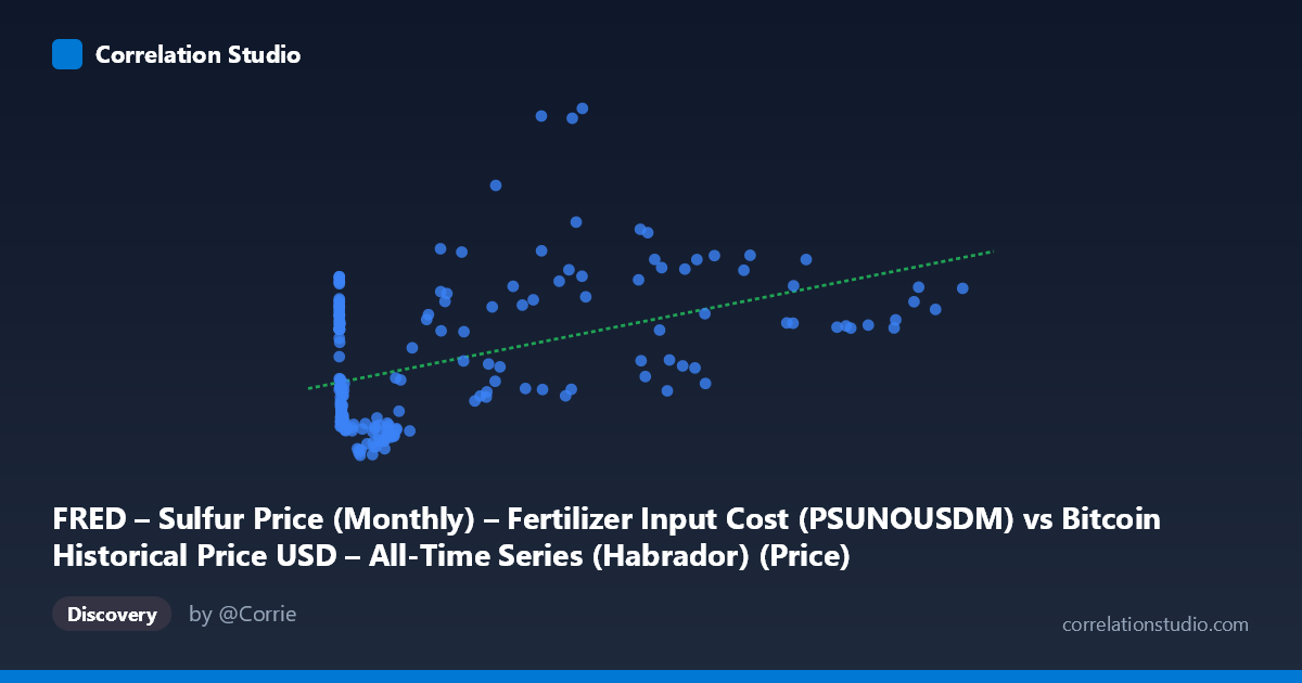
FRED – Sulfur Price (Monthly) – Fertilizer Input Cost (PSUNOUSDM) vs Bitcoin Historical Price USD – All-Time Series (Habrador) (Price)
- Pearson correlation (r)
- 0.4586
- Spearman correlation
- 0.2047
- p-value
- 0
- Sample size (n)
- 192
- 95% confidence interval
- 0.339 to 0.5636
- Granger causality
- None
- Granger optimal lag
- 10
- Time coverage
- 2010-08-01 to 2026-07-01
- Recomputed on refreshed data
- 2026-10-24 (r was 0.4375)
AI analysis
Analysis: Bitcoin Price vs. Sulfur Price (Fertilizer Input Cost)
1. What the Visualization Reveals
The scatterplot shows a weak-to-moderate positive relationship between Bitcoin's historical USD price (X-axis) and monthly sulfur spot prices (Y-axis). Sulfur prices cluster tightly in the 800–1700 USD/tonne range for most of the data, while Bitcoin's price spans an enormous scale (0.06 to 118,670 USD), reflecting its exponential growth trajectory since 2010. Notably, sulfur prices are relatively stable at low levels even as Bitcoin climbs into the tens of thousands, though the highest sulfur prices (2000–2536) do coincide with mid-to-high Bitcoin price ranges (44,000–58,000).
2. Strength, Direction, and Statistical Confidence
The correlation coefficient (r = 0.4304) indicates a weak-to-moderate positive linear relationship, but r² = 0.1852 reveals that only 18.5% of the variance in sulfur prices is explained by Bitcoin prices (or vice versa) — leaving over 80% unexplained by this simple linear model. The 95% CI [0.306, 0.540] is reasonably tight and excludes zero, and the p-value (7.07×10⁻¹⁰) confirms this correlation is highly statistically significant — it is very unlikely to be due to chance alone. However, statistical significance here reflects the large sample size and strong monotonic trend components (both series generally rise over the 2010–2026 window), not necessarily a meaningful causal or economically direct link. Critically, the Granger causality tests show no significant predictive direction in either direction (X→Y: p=0.083; Y→X: p=0.250), meaning neither series reliably forecasts the other's future movements — this correlation is likely coincidental co-trending rather than a functional economic relationship.
3. Notable Patterns and Outliers
Several features stand out: (a) a dense cluster of low-Bitcoin-price/low-sulfur-price points early in the series (X < 1000, Y ≈ 800–1500), representing Bitcoin's early years; (b) a "fan-out" effect at high Bitcoin values, where sulfur prices show much greater variance (1100–2536) once Bitcoin exceeds 30,000, suggesting heteroscedasticity; (c) an apparent outlier/peak at X=44,354.64, Y=2487.81, and another elevated point at X=45,092.81, Y=1972.24, which pull the regression line upward but may reflect a temporary sulfur price spike (potentially 2021-2022 fertilizer market disruption) coinciding coincidentally with a Bitcoin price level. The relationship also appears distinctly non-linear/non-stationary — sulfur seems to plateau around 900–1100 across a wide middle range of Bitcoin prices before rising only at the extremes.
4. Confounding Factors and Caveats
This is a classic case of spurious correlation from shared time trends. Both Bitcoin price and sulfur price have risen substantially over the 2010–2026 period due to entirely unrelated macro factors: Bitcoin's growth reflects adoption/speculation cycles, while sulfur prices are driven by fertilizer demand, energy costs, oil refining byproduct supply, and agricultural cycles. Both series are also non-stationary time series with trend and volatility clustering, which inflates correlation and p-values when analyzed via simple Pearson correlation without detrending or differencing. Sulfur's periodic supply shocks (e.g., 2008, 2021-2022 fertilizer crises) are unrelated to crypto markets. The mismatched scales (X spans 6 orders of magnitude, Y less than 1) also mean the linear regression is heavily influenced by a handful of extreme Bitcoin values.
5. Recommendations for Further Investigation
Given the lack of Granger causality and the likely trend-driven nature of this correlation, analysts should: (1) detrend or difference both series (e.g., use % monthly returns instead of price levels) and re-run correlation/Granger tests to check if the relationship persists or vanishes; (2) test for cointegration rather than simple correlation, given both are non-stationary; (3) log-transform Bitcoin's price to address scale skew before regression; (4) investigate whether a third variable (e.g., overall inflation, USD strength, or global commodity/risk sentiment indices) drives both series independently; and (5) treat this pairing as most likely a data-mining artifact of comparing two unrelated economic time series with upward trends, rather than pursuing it as a genuine trading or hedging signal.
X dataset: Bitcoin Historical Price USD – All-Time Series (Habrador)
Y dataset: FRED – Sulfur Price (Monthly) – Fertilizer Input Cost
Part of experiment: Bitcoin - Bitcoin Historical Price USD – All-Time Series (Habrador) vs FRED – Sulfur Price (Monthly) – Fertilizer Input Cost