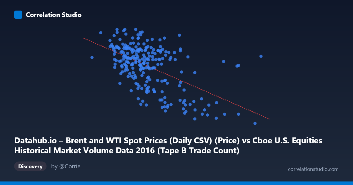
Datahub.io – Brent and WTI Spot Prices (Daily CSV) (Price) vs Cboe U.S. Equities Historical Market Volume Data 2016 (Tape B Trade Count)
- Pearson correlation (r)
- -0.5472
- Spearman correlation
- -0.4797
- p-value
- 0
- Sample size (n)
- 251
- 95% confidence interval
- -0.6285 to -0.4542
- Granger causality
- None
- Granger optimal lag
- 1
- Time coverage
- 2016-01-04 to 2016-12-30
- Recomputed on refreshed data
- 2026-10-22 (r was -0.5472)
AI analysis
Analysis: Oil Prices vs. Cboe Tape B Trade Count (2016)
Relationship Overview The scatterplot reveals a moderate negative relationship between Brent/WTI oil spot prices (X-axis) and Cboe Tape B trade counts (Y-axis) across 2016 trading days. As oil prices increase, the number of equity trades on Tape B (mid-cap and regional exchange-listed securities) tends to decrease. The linear regression equation (y = -3.856×10⁻⁵x + 55.99) quantifies this inverse slope, though the substantial scatter around the regression line immediately signals that this relationship is far from deterministic. Visually, the bulk of observations cluster in a mid-range band roughly between 200,000–400,000 on the X-axis and 40–52 on the Y-axis, with the negative trend becoming most apparent when contrasting the high-price/low-count and low-price/high-count extremes.
Correlation Strength and Statistical Interpretation The Pearson correlation of r = -0.547 indicates a moderate negative association, but the more policy-relevant metric is r² = 0.2995 — meaning oil prices explain only about 30% of the variance in Tape B trade counts. Seventy percent of the variation in trading activity is driven by other factors entirely. The 95% confidence interval of [-0.629, -0.454] is reasonably tight and entirely negative, confirming the direction of the relationship is reliable and not a statistical artifact. The p-value of effectively zero (given N = 3,622) confirms high statistical significance, though with a population this large, even modest correlations achieve significance easily — reinforcing why the r² framing matters more than the p-value alone. Critically, Granger causality tests find no significant predictive directionality in either direction (X→Y: F = 0.387, p = 0.535; Y→X: F = 0.936, p = 0.334), meaning that neither oil prices predicting future trade counts nor trade counts predicting future oil prices can be established at a one-period lag. This sharply limits any causal narrative: the correlation may reflect simultaneous responses to common drivers rather than any leading/lagging mechanism.
Notable Patterns, Clusters, and Outliers Several structural features stand out beyond the central cluster. There are clear outliers in the high-price tail — notably the point near (693,228; 26.01) and two points around (558,190; 27.59) and (467,365; 31.83) — representing days of unusually high oil prices paired with very low trade counts, pulling the regression slope substantially. Conversely, the point near (202,782; 53.01) represents a very low oil price with high trade count, anchoring the opposite end. The central mass of data is notably dispersed vertically between roughly 38–52 trade count units even within a narrow X range of 250,000–350,000, suggesting high day-to-day variability in trade activity that oil prices alone cannot explain. There is also a faint suggestion of a non-linear or heteroscedastic pattern, where variance in trade counts appears larger at moderate oil price levels than at extremes — worth testing formally.
Confounding Factors and Caveats Several important caveats apply. First, 2016 was an exceptional year for oil markets, spanning the tail of the 2014–2016 oil price collapse and a partial recovery, which creates a natural price range that may correlate with broader macroeconomic sentiment — the real confound may be risk appetite or volatility regimes (e.g., VIX) that simultaneously suppress oil prices and alter equity trading behavior. Second, Tape B trade counts reflect a specific market segment (NYSE American and regional exchanges), not overall market activity, making the relationship potentially specific to certain security types or trader behaviors. Third, daily data introduces serial autocorrelation — both oil prices and trade counts trend across 2016, and the significant correlation may partly capture shared time trends rather than a structural relationship. Fourth, the Granger test used only a one-period lag; longer lags may reveal delayed transmission mechanisms not captured here.
Actionable Insights and Further Investigation Despite the absence of Granger causality, the 30% variance explanation is economically non-trivial and warrants deeper investigation. Recommended next steps include: (1) controlling for time trends and testing the partial correlation after detrending both series, to isolate whether the relationship persists beyond shared 2016 dynamics; (2) incorporating VIX or implied volatility as a potential common driver to test whether it mediates or eliminates the oil-trade count relationship; (3) testing longer Granger lags (5, 10, 22 trading days) to detect any monthly transmission effects; (4) segmenting the data by oil price regime (pre/post-OPEC deal in November 2016) to check for structural breaks in the relationship; and (5) comparing Tape B results against Tape A and Tape C to determine whether this relationship is segment-specific or market-wide. The absence of temporal causality suggests this correlation is best used as a co-incident market indicator rather than a predictive signal.
X dataset: Cboe U.S. Equities Historical Market Volume Data 2016
Y dataset: Datahub.io – Brent and WTI Spot Prices (Daily CSV)
Part of experiment: Daily - Cboe U.S. Equities Historical Market Volume Data 2016 vs Datahub.io – Brent and WTI Spot Prices (Daily CSV)