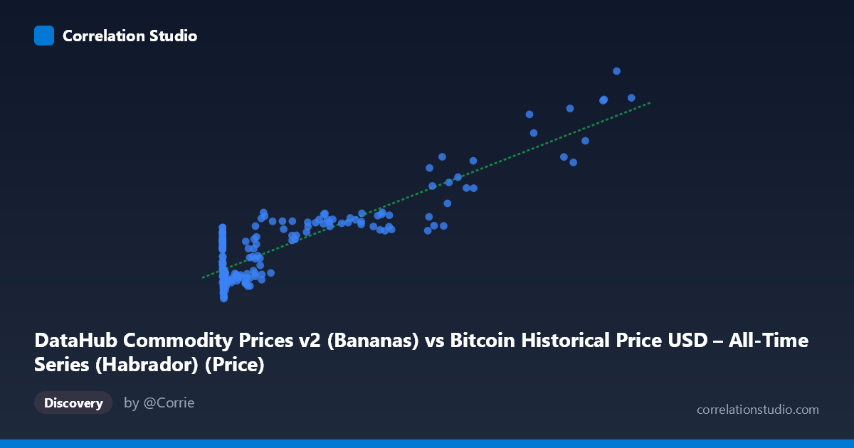
DataHub Commodity Prices v2 (Bananas) vs Bitcoin Historical Price USD – All-Time Series (Habrador) (Price)
- Pearson correlation (r)
- 0.891
- Spearman correlation
- 0.6143
- p-value
- 0
- Sample size (n)
- 182
- 95% confidence interval
- 0.8566 to 0.9175
- Granger causality
- None
- Granger optimal lag
- 4
- Time coverage
- 2010-08-01 to 2025-09-01
- Recomputed on refreshed data
- 2026-10-24 (r was 0.891)
AI analysis
Analysis: Bitcoin Price vs. Banana Commodity Prices
1. What the Visualization Reveals
This scatterplot juxtaposes Bitcoin's historical USD price against a banana commodity price index — two economically unrelated series that happen to show a strong statistical association. The data reveals a clear monotonic, curved (logarithmic-like) relationship: at low Bitcoin prices (under ~$1,000), the "Y" values cluster tightly between 85–145, while as Bitcoin climbs into the tens of thousands, Y rises correspondingly toward 150–280. The shape is not linear in the traditional sense — it resembles a log or power curve, since Y compresses at low X and spreads out more gradually at high X despite X spanning nearly 6 orders of magnitude (0.06 to 113,500).
2. Strength, Direction, and Statistical Meaning
The correlation is strong and positive (r = 0.891), with r² = 0.794 indicating that roughly 79% of the variance in Y is statistically explainable by X. The 95% CI [0.857, 0.918] is tight and the p-value is effectively zero, so the correlation itself is not a fluke of sampling — it is a robust, reproducible pattern in this dataset. However, statistical significance here should not be mistaken for causal or mechanistic linkage. The Granger causality tests are decisive on this point: neither direction shows predictive power (X→Y: p=0.82; Y→X: p=0.97). This means past Bitcoin prices do not help forecast future banana prices, and vice versa. The correlation is almost certainly driven by a shared underlying trend — both series have risen over the 2010–2025 window (Bitcoin due to adoption/speculation, commodity indices due to inflation/monetary expansion) — rather than any economic interaction between crypto markets and banana prices.
3. Notable Patterns and Features
The scatter shows a distinctive "hockey-stick" or log-curve shape rather than a straight line, suggesting the linear R²=0.794 may actually understate the fit quality of a log-transformed model (log(X) vs Y would likely show an even tighter, more linear relationship given the multi-order-of-magnitude spread in X). There's a dense cluster of low-X, low-Y points (X < 50,000, Y in 85–160 range) corresponding to Bitcoin's early years, and a sparser upper tail (X 90,000) where Y climbs to 200–280 — these are recent high-price Bitcoin periods. No extreme outliers break the general trend, though there's some vertical scatter at mid-range X values (e.g., X≈9,000–46,000 shows Y ranging from ~104 to ~160), indicating that at any given Bitcoin price level, banana prices vary due to their own independent dynamics (seasonality, weather, trade policy).
4. Confounding Factors and Caveats
This is a textbook case of spurious correlation via co-trending time series. Both variables are non-stationary and generally trend upward over the 15-year window, so almost any two "monotonically increasing over time" series would show high correlation without any real link. Likely confounders include: global inflation/USD purchasing power, general macroeconomic growth, and the mere passage of time. The mismatched sampling frequency (Bitcoin is continuous/daily; commodity prices are monthly) and the dataset's odd cross-listing (each column drawn from a different dataset than its label suggests) also raise data-integrity concerns worth double-checking before drawing conclusions.
5. Actionable Insights
- Do not use this correlation for trading or forecasting — Granger results confirm no predictive temporal relationship exists. - De-trend or difference both series (e.g., use % changes or returns rather than levels) and recompute correlation; this is the standard remedy for spurious trend-driven correlation and would likely show r near zero. - Try log(X) vs Y regression — given the curve shape, this will likely improve fit and better characterize the true functional relationship, if one is deemed worth reporting at all. - Treat this pairing as an illustrative example of "correlation without causation," useful for pedagogical purposes on time-series pitfalls rather than genuine economic insight.
X dataset: Bitcoin Historical Price USD – All-Time Series (Habrador)
Y dataset: DataHub Commodity Prices v2
Part of experiment: Bitcoin - Bitcoin Historical Price USD – All-Time Series (Habrador) vs DataHub Commodity Prices v2