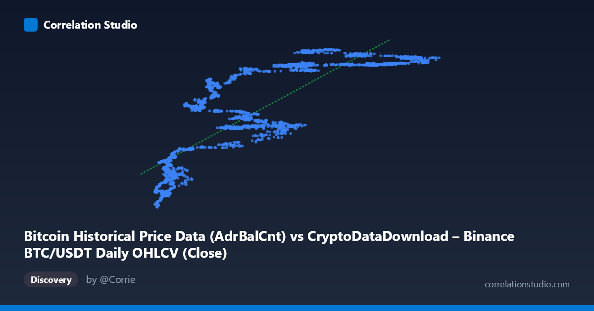
Bitcoin Historical Price Data (AdrBalCnt) vs CryptoDataDownload – Binance BTC/USDT Daily OHLCV (Close)

Pearson correlation (r): 0.8285
Spearman correlation: 0.8984
p-value: 0
Sample size (n): 3191
95% confidence interval: 0.8173 to 0.8391
Granger causality: None
Granger optimal lag: 10
Time coverage: 2017-08-17 to 2026-05-20

AI analysis

Analysis of Bitcoin Address Balance Count vs. BTC/USDT Close Price

1. What the Visualization Reveals

The scatterplot depicts a positive, moderately strong relationship between the number of Bitcoin addresses holding a balance (AdrBalCnt) and the daily closing price of BTC/USDT. As the address count grows from roughly 3,000 to 125,000 (units unspecified but likely thousands, given typical AdrBalCnt scaling), closing prices trend upward from the high-teens millions to the mid-50-millions (again, likely a scaled or indexed price representation). The pattern is clearly upward-sloping but shows considerable dispersion, particularly in the low-to-mid X range, suggesting the relationship is real but noisy rather than deterministic.

2. Strength, Direction, and Statistical Confidence

The correlation coefficient (r = 0.83) indicates a strong positive linear association, with r² = 0.686 meaning roughly 69% of the variance in closing price is statistically explained by variance in address balance count — leaving about 31% attributable to other factors, noise, or nonlinear dynamics. The 95% confidence interval [0.817, 0.839] is tight, and the p-value is effectively zero, so we can be highly confident this correlation is not a statistical fluke — it's a robust, reproducible pattern in this sample. However, the Granger causality tests complicate the causal story: neither direction reaches significance at conventional thresholds (X→Y: p = 0.156; Y→X: p = 0.051, only marginally short of significance). This means neither variable reliably predicts the other's future movements in a time-lagged sense, despite their strong contemporaneous correlation. Practically, this suggests both series may be driven by a common underlying factor (e.g., overall market adoption/growth trends) rather than one directly causing the other.

3. Notable Patterns and Non-linear Features

Several structural features stand out. First, there's a visible "floor" cluster at low X values (roughly 3,000–15,000) where Y ranges widely from ~19M to ~31M — this vertical spread suggests high price volatility when address counts are low, possibly corresponding to early market history or bear-market accumulation phases. Second, a mid-range plateau appears between X ≈ 50,000–90,000 where Y clusters tightly around 51M–57M, hinting at a saturation effect or a price ceiling/consolidation zone. Third, some points (e.g., X≈24,712 with Y≈33.2M, or X≈54,884 with Y≈36.4M) fall noticeably below the general trend line, indicating periods where price growth lagged address growth — potentially bear markets or corrections. The overall shape hints at a logarithmic or S-curve relationship rather than pure linearity, since price growth appears to decelerate relative to address growth at the high end.

4. Confounding Factors and Caveats

This analysis carries important caveats. Both series are time-ordered (2017–2026) and likely non-stationary — Bitcoin price and adoption metrics both trend upward over time due to secular market growth, which can produce spurious correlation even absent direct causation. Address count itself can be inflated by exchange consolidation practices, dust transactions, or address reuse patterns unrelated to genuine organic adoption. Additionally, macroeconomic factors (interest rates, regulatory news, halving cycles, exchange listings) likely drive both variables simultaneously, which would explain the strong correlation coupled with the lack of clear Granger causality — a classic sign of confounding by a shared latent trend rather than direct predictive linkage.

5. Actionable Insights and Further Investigation

Given the non-stationarity concern, I'd recommend re-running the correlation and Granger tests on differenced or detrended series (e.g., daily returns/changes rather than levels) to check whether the relationship holds after removing shared trend components — this is standard practice to avoid spurious regression in time series. It would also be valuable to segment the analysis by market regime (bull vs. bear phases) to see if the relationship strength or slope changes, given the plateau and outlier clusters observed. Finally, since the Y→X Granger test is only marginally non-significant (p=0.051), a slightly longer lag window or alternate lag-selection criterion might reveal that price changes modestly precede address count changes — worth testing at multiple lag lengths (5, 15, 20 periods) to check robustness of the "no causality" conclusion.

X dataset: CryptoDataDownload – Binance BTC/USDT Daily OHLCV

Y dataset: Bitcoin Historical Price Data

Part of experiment: Bitcoin - CryptoDataDownload – Binance BTC/USDT Daily OHLCV vs Bitcoin Historical Price Data