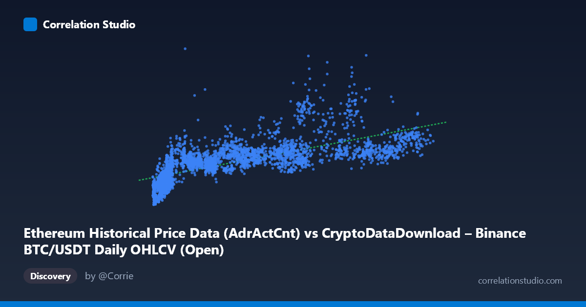
Ethereum Historical Price Data (AdrActCnt) vs CryptoDataDownload – Binance BTC/USDT Daily OHLCV (Open)
- Pearson correlation (r)
- 0.6958
- Spearman correlation
- 0.8291
- p-value
- 0
- Sample size (n)
- 3191
- 95% confidence interval
- 0.6775 to 0.7133
- Granger causality
- None
- Granger optimal lag
- 10
AI analysis
Scatterplot Analysis: BTC/USDT Metrics vs. Ethereum Price Data
1. Relationship Overview
The visualization depicts a moderate positive relationship between the X variable (labeled as Ethereum AdrActCnt, though contextually appears to be BTC-related given the dataset source) and Y (BTC/USDT Open price). As X increases from roughly 3,000 to 125,000, Y tends to rise as well — from the 130K–200K range at low X values up toward 600K–1.5M at higher X values. However, the spread around this trend is substantial, particularly in the middle-to-upper X range (40,000–90,000), where Y values scatter widely between ~440,000 and ~1,000,000 for similar X inputs. This indicates a real but noisy association rather than a tight linear coupling.
2. Strength, Direction, and Statistical Confidence
The Pearson correlation of r = 0.696 indicates a moderate-to-strong positive linear relationship, but r² = 0.484 is the more practically important figure: only 48.4% of the variance in Y is explained by X, leaving over half unexplained by this single predictor. The 95% confidence interval [0.678, 0.713] is narrow and does not cross zero, and the p-value of effectively 0 confirms this correlation is highly statistically significant (unsurprising given n = 3,191) — but statistical significance here reflects sample size more than practical predictive strength. Critically, the Granger causality tests show no significant predictive direction in either direction (X→Y: p=0.71; Y→X: p=0.64) even at an optimal lag of 10 periods. This means that despite the contemporaneous correlation, neither series reliably helps forecast the other's future values — the relationship is likely driven by a shared underlying trend (e.g., both being tied to overall crypto market cycles) rather than one variable causing or leading the other.
3. Patterns, Clusters, and Non-linear Features
Several structural features stand out: - Low-X cluster (X < 15,000): Y values are compressed into a lower band (~140,000–500,000), suggesting a floor effect or early-period data (likely 2017–2019 bear/early market). - Fan-shaped divergence: As X grows beyond ~50,000, the vertical spread of Y widens dramatically (e.g., X≈68,000 pairs with Y=999,185, while X≈70,780 pairs with Y=642,512), indicating heteroscedasticity — variance in Y is not constant across X. - High-Y outliers: Points like (68113.92, 999185.00) and (80905.53, 936565.00) sit well above the regression line, hinting at a possible secondary regime (e.g., bull-market spikes) not captured by a single linear fit. - The note that Spearman ρ exceeds Pearson r confirms curvature — a logarithmic or power-law fit (common in price/volume or price/adoption relationships) likely captures the relationship better than the straight line y = 3.85x + 357,008.
4. Confounding Factors and Caveats
The X and Y labels reference mismatched datasets (Ethereum AdrActCnt vs. Binance BTC/USDT Open), so it's unclear whether this is truly ETH-activity-vs-BTC-price or a labeling artifact — this should be clarified before drawing asset-specific conclusions. More importantly, both series span 2017–2026, a period encompassing multiple bull/bear cycles, halving events, and macro shocks (COVID, rate hikes, regulatory news). Since both crypto prices and on-chain activity metrics tend to trend together with overall market sentiment, this is a classic case of spurious/confounded correlation via a common time trend rather than a direct causal link — reinforced by the null Granger causality result. Autocorrelation within each time series (non-independent observations) also inflates apparent significance and violates i.i.d. assumptions underlying the p-value calculation.
5. Recommendations for Further Investigation
1. Verify variable labeling — confirm whether X and Y are genuinely cross-asset (ETH activity vs. BTC price) or a data-pipeline mismatch. 2. Detrend or difference the series (e.g., use returns/log-differences instead of levels) before correlation/Granger testing to remove spurious trend-driven correlation. 3. Fit a log-log or polynomial model given the Spearman/Pearson discrepancy — this could substantially raise explained variance. 4. Segment by market regime (bull vs. bear, halving cycles) to see if the relationship is stable or regime-dependent, given the visible fan/heteroscedastic pattern. 5. Since Granger tests show no lead-lag predictability, this pairing should not be used for forecasting one variable from the other; treat the correlation as descriptive/co-movement evidence only, not a trading or predictive signal.
X dataset: CryptoDataDownload – Binance BTC/USDT Daily OHLCV
Y dataset: Ethereum Historical Price Data
Part of experiment: Bitcoin - CryptoDataDownload – Binance BTC/USDT Daily OHLCV vs Ethereum Historical Price Data