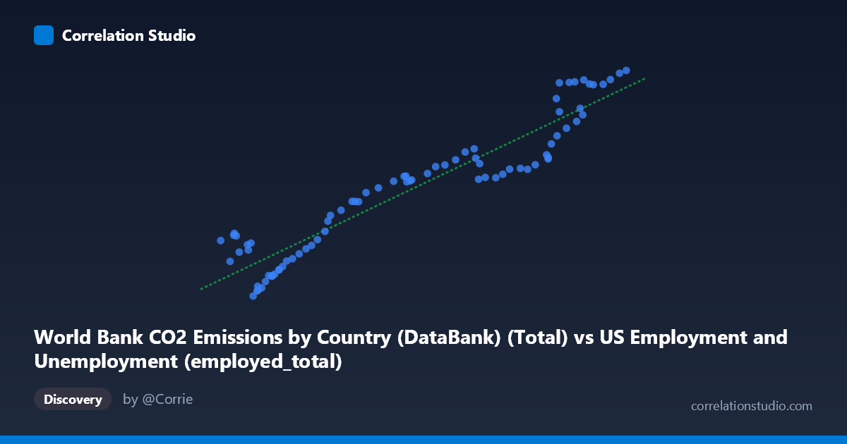
World Bank CO2 Emissions by Country (DataBank) (Total) vs US Employment and Unemployment (employed_total)
- Pearson correlation (r)
- 0.945
- Spearman correlation
- 0.9313
- p-value
- 0
- Sample size (n)
- 80
- 95% confidence interval
- 0.9154 to 0.9645
- Granger causality
- None
- Granger optimal lag
- 10
- Time coverage
- 1941-01-01 to 2020-01-01
AI analysis
Scatterplot Analysis: US Total Employment vs. World Bank CO2 Emissions
Relationship Overview
The scatterplot reveals a strong, positive relationship between total US employment figures and CO2 fossil fuel emissions, with data spanning 1941–2020. As employment rises, CO2 emissions increase in a broadly consistent pattern, and the linear regression model (y = 0.2647x − 1060.42) fits the data reasonably well across much of the range. The upward sweep of points from lower-left to upper-right is visually pronounced, reflecting nearly eight decades of parallel growth in both workforce size and carbon output — a pattern consistent with economic expansion driving both labor demand and energy consumption simultaneously.
Correlation Strength and Statistical Interpretation
The Pearson correlation of r = 0.945 is statistically very strong, and with p ≈ 0, the probability of observing this association by chance under the null hypothesis is negligible. The R² of 0.893 means that approximately 89.3% of the variance in CO2 emissions is statistically explained by variation in total employment — a remarkably high figure for a social-environmental cross-dataset comparison. The 95% confidence interval for r of [0.915, 0.965] is narrow, indicating high precision and stability in this estimate across plausible samples. However, the Granger causality results tell an important cautionary story: neither X→Y (F = 0.889, p = 0.550) nor Y→X (F = 0.903, p = 0.538) reaches significance at any conventional threshold, even with an optimal lag of 10 periods. This means that neither variable temporally predicts the other beyond their shared trend — a strong signal that the high correlation is driven by a common underlying driver (likely long-run economic and population growth) rather than any direct causal mechanism between employment and emissions.
Notable Patterns, Clusters, and Outliers
Several structural features are visible in the data. At lower employment values (roughly 50,000–75,000 on the X-axis), there is notable vertical scatter — multiple Y values cluster at similar emissions levels despite varying employment, suggesting these earlier decades had less predictable relationships. In the mid-range (X ≈ 85,000–130,000), the data points align most tightly with the regression line, forming the most coherent linear segment. In the upper range (X 140,000), there is a visible fan-shaped divergence, with several high-employment observations yielding a wide spread of emissions outcomes — some considerably above and others below the regression line. A few points, such as (50,350; 18,044) and (53,960; 19,109), appear as potential outliers sitting above the regression line at low employment values, possibly reflecting wartime or early postwar anomalies in the 1940s where industrial emissions were high relative to civilian workforce size.
Confounding Factors and Caveats
The most fundamental caveat here is that both variables are time-indexed series growing over the same 80-year span, making spurious correlation through shared temporal trend the leading concern. Any two quantities that generally increase from 1941 to 2020 — population, GDP, energy use, vehicle registrations — would likely produce a similarly high r. The Granger non-causality result reinforces this: the correlation is not mechanistically informative. Additionally, structural breaks — the 2008–2009 financial crisis, the COVID-19 shock of 2020, and major energy transitions — may influence specific data points without being visible in aggregate. The dataset mixing of "US employment" with "World Bank global CO2" also raises a scope mismatch concern: US employment is a domestic labor measure, while the CO2 dataset is multinational, potentially introducing noise from non-US emissions trajectories embedded in the Y variable.
Actionable Insights and Further Investigation
Given the strength of the correlation but the absence of Granger causality, further investigation should focus on isolating the shared driver rather than treating this as a bilateral relationship. Researchers should consider: (1) partialing out GDP or population as control variables to test whether a residual employment–emissions relationship persists; (2) examining sector-specific employment (manufacturing, transportation, energy) against US-only CO2 data to test more mechanistically plausible links; (3) applying structural break tests around key dates (1973 oil shock, 2008 recession, 2016 energy mix shifts) to assess whether the linear relationship is stable or regime-dependent; and (4) extending Granger tests with shorter lags or alternative causality frameworks (e.g., transfer entropy) given that 10-period lags may be too long to detect short-run predictive dynamics in annual data. The high R² is analytically interesting but should not be interpreted as policy-relevant without resolving the confounding structure.
X dataset: US Employment and Unemployment
Y dataset: World Bank CO2 Emissions by Country (DataBank)
Part of experiment: Yearly - US Employment and Unemployment vs World Bank CO2 Emissions by Country (DataBank)