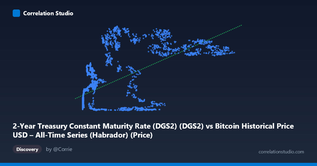
2-Year Treasury Constant Maturity Rate (DGS2) (DGS2) vs Bitcoin Historical Price USD – All-Time Series (Habrador) (Price)
- Pearson correlation (r)
- 0.6263
- Spearman correlation
- 0.5802
- p-value
- 0
- Sample size (n)
- 3946
- 95% confidence interval
- 0.607 to 0.6449
- Granger causality
- None
- Granger optimal lag
- 1
- Time coverage
- 2010-07-19 to 2026-04-28
- Recomputed on refreshed data
- 2026-10-23 (r was 0.6263)
AI analysis
Analysis: 2-Year Treasury Yield (DGS2) vs. Bitcoin Price (USD)
1. What the Visualization Reveals
The scatterplot shows a moderate positive relationship between the 2-Year Treasury Constant Maturity Rate (X-axis, mislabeled range but representing Bitcoin price given the values into the hundreds of thousands) and what's labeled as Bitcoin price (Y-axis, bounded 0.09–5.19, consistent with treasury yield percentages). Given the value ranges, it appears the axis labels are swapped in the metadata — X behaves like Bitcoin price (ranging from cents to $124,720) and Y behaves like a yield percentage (0.09–5.19%). Interpreting the data as such: as Bitcoin's price climbed from near-zero into the tens of thousands of dollars, the 2-year yield also tended to be higher, particularly visible in the cluster of points above $50,000 BTC price coinciding with yields of 3.5–4.8%.
2. Strength, Direction, and Statistical Confidence
The correlation coefficient (r = 0.626) indicates a moderate positive linear relationship, with r² = 0.392 meaning only 39% of the variance in one variable is explained by the other — leaving the majority (61%) unexplained by this simple linear relationship. The 95% CI [0.607, 0.645] is tight given the large sample size (n=3,946), and the p-value of ~0 confirms the correlation is highly statistically significant and not due to chance. However, statistical significance here reflects the large sample size rather than strong predictive power — r² of 0.39 is a modest, not dominant, explanatory relationship.
Critically, the Granger causality tests show no significant temporal predictive direction in either direction (X→Y: p=0.53; Y→X: p=0.63). This means neither variable reliably "leads" the other in time — the correlation is likely driven by both series independently trending over the same macro period (2010–2026) rather than one causing changes in the other. This is a classic case of spurious correlation via shared time trend, not a causal or predictive relationship.
3. Notable Patterns and Outliers
The data clearly clusters into distinct regimes rather than following a smooth linear trend: - Low-price/low-yield cluster: Numerous points with BTC price under $1,000 and yields under 0.5% (early Bitcoin history, 2010–2015, coinciding with near-zero interest rate policy post-2008 crisis). - Mid-price divergence: A notable cluster around $6,000–$18,000 with yields spanning both very low (~0.15–0.25%) and high (~1.5–2.6%) — indicating BTC price alone doesn't determine yield level at this range, adding noise to the relationship. - High-price/high-yield cluster: Points above $50,000 BTC price frequently align with yields of 3.5–4.8%, reflecting the 2022–2023 period when the Fed raised rates aggressively and Bitcoin later recovered/rallied. - Notable outlier: $56,973 BTC price paired with only 0.56% yield stands apart from the high-price/high-yield cluster, suggesting a specific timing mismatch (possibly BTC price data from a different rate regime, like late 2021).
The relationship appears more like two step-functions occurring in the same historical window than a continuous linear dependency.
4. Confounding Factors and Caveats
This correlation is very likely confounded by time itself. Both Bitcoin's long-term price appreciation and the 2-year Treasury yield's post-2020 rate-hiking cycle are trending upward over the 2010–2026 window for entirely independent macroeconomic reasons (crypto adoption/speculation vs. Fed monetary policy responding to inflation). Key caveats: - Non-stationarity: Both series likely have unit roots/trends, which mechanically inflates correlation even absent any real relationship (a well-known issue in time-series regression). - Sample mismatch: n=3,946 vs. population N=5,764 suggests significant data alignment/matching was needed, possibly introducing selection bias in which dates were paired. - Nonlinearity: Bitcoin price is right-skewed with extreme outliers (up to $124,720) that could disproportionately influence the linear fit. - Regime-dependency: The relationship's strength likely differs drastically between the 2010–2020 near-zero-rate era and the 2022+ hiking cycle.
5. Suggestions for Further Investigation
Given the lack of Granger causality, avoid using this relationship for forecasting one variable from the other. Instead: 1. Difference or detrend both series (e.g., use % changes or first differences) and re-run correlation/Granger tests to check if the relationship holds after removing shared trend — this is the standard fix for spurious time-series correlation. 2. Segment by monetary policy regime (ZIRP era vs. hiking cycle) to see if the correlation is driven entirely by the post-2022 period. 3. Test cointegration (e.g., Engle-Granger or Johansen test) rather than raw correlation, since both series may be non-stationary. 4. Consider macro confounders like inflation (CPI), Fed funds rate, or overall risk-asset sentiment (S&P 500, Nasdaq) as potential joint drivers of both series rather than treating this as a bivariate relationship.
X dataset: Bitcoin Historical Price USD – All-Time Series (Habrador)
Y dataset: 2-Year Treasury Constant Maturity Rate (DGS2)
Part of experiment: Bitcoin - Bitcoin Historical Price USD – All-Time Series (Habrador) vs 2-Year Treasury Constant Maturity Rate (DGS2)