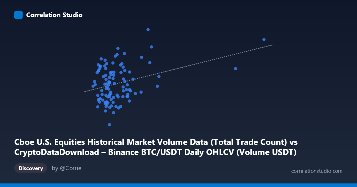
Cboe U.S. Equities Historical Market Volume Data (Total Trade Count) vs CryptoDataDownload – Binance BTC/USDT Daily OHLCV (Volume USDT)
- Pearson correlation (r)
- 0.3309
- Spearman correlation
- 0.1612
- p-value
- 0.000602
- Sample size (n)
- 104
- 95% confidence interval
- 0.1477 to 0.4921
- Granger causality
- None
- Granger optimal lag
- 10
- Time coverage
- 2026-01-02 to 2026-06-25
- Recomputed on refreshed data
- 2026-10-22 (r was 0.3309)
AI analysis
Analysis: Cboe Equities Trade Count vs. Binance BTC/USDT Volume (USDT)
1. Overall Relationship The scatterplot shows a positive but noisy relationship between two variables from entirely unrelated market ecosystems: U.S. equities trade counts (Cboe) and Binance BTC/USDT dollar trading volume. The data cloud shows a general upward drift — as X (equities trade count) increases, Y (crypto volume) also tends to increase — but the scatter is wide, with most points clustered tightly on the low-X end (under ~2 billion) and a handful of high-X outliers stretching the trend line.
2. Strength, Direction, and Statistical Meaning The correlation (r = 0.448) is moderate in strength, and r² = 0.20 indicates that only about 20% of the variance in Binance trading volume is statistically associated with variance in Cboe trade counts — leaving 80% unexplained by this single variable. The 95% CI [0.265, 0.599] is fairly wide, reflecting real sampling uncertainty even though the p-value (9.7×10⁻⁶) confirms the correlation is unlikely due to chance at n=90. Critically, the Granger causality tests show no significant predictive direction in either direction (X→Y p=0.436; Y→X p=0.636), meaning that despite the contemporaneous correlation, neither series meaningfully forecasts the other over time. This strongly suggests the relationship is either coincidental, driven by a shared external factor (e.g., overall market activity growth, calendar effects, or macro liquidity trends), or simply a spurious correlation between two unrelated volume metrics that both trend upward over the observation period.
3. Patterns, Clusters, and Outliers The data is heavily right-skewed on the X-axis: the bulk of points (roughly 80+ of 90) fall between 800M–2.5B trades, while a small number of extreme outliers (e.g., X ≈ 7.2B, 6.1B, 3.2B) sit far to the right. These few high-leverage points likely have outsized influence on the regression slope and the correlation coefficient — removing them could substantially change r and r². Within the main cluster, Y values range broadly (roughly 5.2M–9.4M) with no clear sub-clustering or nonlinear curvature, suggesting the "relationship" within the dense cloud is closer to noise, and much of the apparent correlation is being pulled by the sparse tail of large-X points.
4. Confounding Factors and Caveats This pairing is conceptually unusual: it compares U.S. equities market trade counts to crypto exchange dollar volume — two markets with different participants, drivers, and time dynamics (e.g., equities trade during market hours; crypto trades 24/7). Any correlation is more likely explained by shared temporal trends (both markets growing/volatile over the Jan–May 2026 window), general market-wide risk sentiment, or coincidental co-movement rather than any direct economic linkage. Additionally, with only 90 sampled points from a population of 1,980, and heavy skew/leverage from a few extreme X values, the r² and r estimates are fragile and sensitive to outlier removal or resampling.
5. Suggestions for Further Investigation - Test robustness: Recompute correlation with the extreme high-X outliers removed or winsorized to see if r² holds up in the dense cluster. - Log-transform X: Given the strong right-skew, a log(X) transformation may reveal a cleaner, more linear (or reveal a nonexistent) relationship. - Investigate confounders: Check whether both series correlate independently with a plausible shared driver (e.g., date/time trend, VIX, overall trading-day volume growth, or macro liquidity indices). - Treat causally with caution: Given the lack of Granger causality, avoid using one series to forecast the other; the correlation should be treated as descriptive/associative only, not predictive. - Extend time series: With N=1,980 available but only 90 sampled, using the full dataset (or a larger, non-uniform sample) would yield tighter confidence intervals and a more reliable causality test.
X dataset: CryptoDataDownload – Binance BTC/USDT Daily OHLCV
Y dataset: Cboe U.S. Equities Historical Market Volume Data
Part of experiment: Bitcoin - CryptoDataDownload – Binance BTC/USDT Daily OHLCV vs Cboe U.S. Equities Historical Market Volume Data