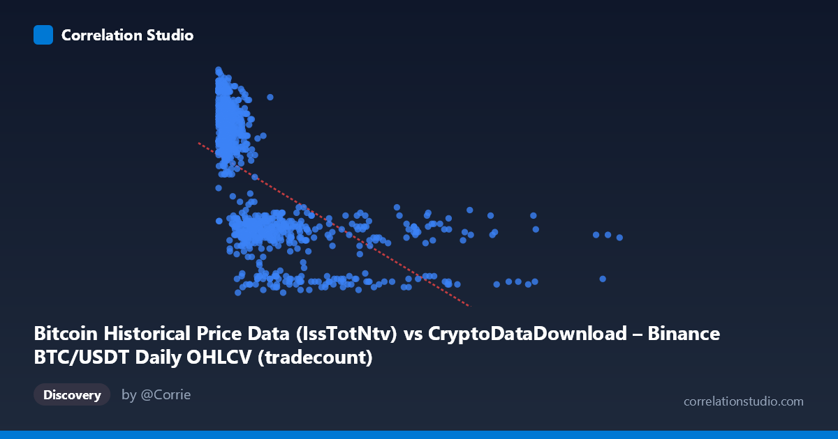
Bitcoin Historical Price Data (IssTotNtv) vs CryptoDataDownload – Binance BTC/USDT Daily OHLCV (tradecount)
- Pearson correlation (r)
- -0.5883
- Spearman correlation
- -0.7608
- p-value
- 0
- Sample size (n)
- 938
- 95% confidence interval
- -0.6286 to -0.5448
- Granger causality
- None
- Granger optimal lag
- 10
- Time coverage
- 2017-08-20 to 2026-05-20
AI analysis
Analysis of Bitcoin Volume Metric vs. Trade Count Relationship
1. What the Visualization Reveals
The scatterplot shows a clear negative relationship between the X-axis metric (appears to be a volume/native-units measure, labeled "IssTotNtv") and tradecount (Y-axis). As X increases, Y systematically decreases, but the relationship is distinctly curved rather than linear — the data shows a steep drop at low X values (roughly 0–1M) followed by a long, flattening tail as X extends into the millions. Points with very high X values (5M–12M) cluster tightly at low Y values (400–500 tradecount range), while the bulk of variance and scatter occurs in the lower X range where Y spans from ~700 to ~2300.
2. Strength, Direction, and Statistical Confidence
The Pearson correlation of r = -0.588 indicates a moderate-to-strong negative linear association, with r² = 0.346 meaning only about 35% of the variance in tradecount is explained by this X variable under a linear model — leaving nearly two-thirds unexplained. The 95% CI [-0.629, -0.545] is narrow and does not cross zero, and the p-value of 0 confirms this correlation is highly statistically significant, not a product of chance, given the large sample (n=938). However, statistical significance should not be conflated with practical predictive power — r² of 0.35 leaves substantial room for other drivers of tradecount. Critically, the Granger causality tests show no significant temporal predictive direction in either direction (X→Y: p=0.44; Y→X: p=0.58), meaning past values of one series do not reliably forecast future values of the other. This suggests the correlation is likely contemporaneous/structural (e.g., both driven by market regime or price level) rather than one variable causally leading the other over time.
3. Notable Patterns and Non-linear Features
The most important feature is the curvature: this looks like an inverse or logarithmic decay relationship rather than a straight line. Low-X observations (under ~500K) show high Y values with substantial spread (1600–2300), while X values above ~3M compress into a narrow low-Y band. This is consistent with the note that Spearman ρ exceeds Pearson r — a log transformation of X (e.g., log(X) vs. Y) would likely produce a much stronger linear fit and higher R². There also appears to be a possible secondary cluster or regime shift — the very high X points (5.7M, 6.9M, 9M+) behave almost as a separate low-variance group, possibly corresponding to distinct market periods (e.g., specific dates with anomalously high issuance/volume values) rather than a continuous relationship with the bulk of the data.
4. Confounding Factors and Caveats
Both variables are derived from the same underlying BTC/USDT trading activity, so this may reflect shared market mechanics rather than an independent causal link — e.g., during high-volatility periods, both trade volume and trade count could move together or inversely due to changes in average trade size, algorithmic trading behavior, or exchange fee structures. The time span (2017–2026) covers multiple market cycles (bull runs, crashes, halving events), so temporal non-stationarity is a serious concern — the relationship may not be stable across regimes, and pooling all periods into one correlation could mask regime-specific dynamics. Additionally, "IssTotNtv" is an unusual/ambiguous metric name — its exact definition (native token issuance? cumulative volume?) should be verified before drawing economic conclusions, since mismeasurement or unit inconsistencies could distort the relationship.
5. Suggested Next Steps
1. Refit with a log or power transformation on X (given the Spearman/Pearson divergence) to better capture the apparent non-linear decay and improve explained variance. 2. Segment the analysis by time period or market regime (e.g., bull vs. bear markets, pre/post-halving) to check whether the negative relationship is stable or driven by a few extreme episodes (the 5M+ X cluster). 3. Investigate the exact definition of "IssTotNtv" to ensure it's not mechanically related to tradecount (e.g., a derived or overlapping metric), which could inflate the correlation artificially. 4. Given the lack of Granger causality, treat this as a descriptive/structural correlation, not a forecasting signal — avoid using one variable to predict future values of the other in trading models without further validation. 5. Consider multivariate analysis incorporating price, volatility, or volume-per-trade to identify true drivers of tradecount rather than relying on this bivariate relationship alone.
X dataset: CryptoDataDownload – Binance BTC/USDT Daily OHLCV
Y dataset: Bitcoin Historical Price Data
Part of experiment: Bitcoin - CryptoDataDownload – Binance BTC/USDT Daily OHLCV vs Bitcoin Historical Price Data