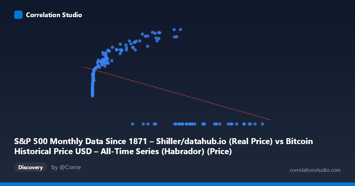
S&P 500 Monthly Data Since 1871 – Shiller/datahub.io (Real Price) vs Bitcoin Historical Price USD – All-Time Series (Habrador) (Price)
- Pearson correlation (r)
- -0.4567
- Spearman correlation
- 0.0113
- p-value
- 0
- Sample size (n)
- 194
- 95% confidence interval
- -0.5615 to -0.3376
- Granger causality
- None
- Granger optimal lag
- 10
- Time coverage
- 2010-08-01 to 2026-09-01
- Recomputed on refreshed data
- 2026-10-24 (r was -0.4161)
AI analysis
Analysis: Bitcoin Price vs. S&P 500 (Real Price) Relationship
1. What the Visualization Reveals
The scatterplot shows a scattered, non-linear pattern rather than a clean linear relationship. At low X values (roughly 0–1,000), Y values cluster tightly between ~1,500–3,000, showing a steep rise as X increases from near-zero. However, at high X values (50,000), Y frequently collapses to 0, creating a bifurcated pattern: one cluster of moderate-to-high Y values at low-to-mid X, and a separate cluster of zero Y values scattered across the entire high-X range. This suggests the data is not truly bivariate-continuous but instead reflects two different regimes or a data artifact (e.g., missing/zero-filled values for one series during certain time periods).
2. Strength, Direction, and Statistical Confidence
The correlation coefficient (r = -0.416) indicates a moderate negative relationship, but r² = 0.173 tells the more important story: only 17.3% of the variance in Y is explained by X — meaning over 80% of Y's variability is driven by other factors. The 95% CI [-0.528, -0.291] is reasonably tight and excludes zero, and the p-value (2.6×10⁻⁹) confirms this correlation is statistically significant and not due to chance. However, statistical significance ≠ practical strength — this is a weak-to-moderate relationship, not one suitable for precise prediction. The Granger causality tests are notably inconclusive: neither X→Y (p=0.167) nor Y→X (p=0.065) reaches significance at the 0.05 threshold, meaning neither series reliably predicts the other's future movements in a temporal sense, despite lag testing up to 10 periods. This undermines any causal or forecasting narrative.
3. Notable Patterns and Outliers
The most striking feature is the zero-inflation at high X values — numerous points where Y=0 occur specifically when X exceeds ~27,000, while Y is always positive (1,500–5,140) when X is low. This is not a smooth negative trend but rather looks like a structural break or regime shift, possibly indicating that once X (labeled as "S&P 500 Real Price" but seemingly containing Bitcoin-scale values) crosses a threshold, the corresponding Y data becomes unavailable, zero-filled, or represents a different market condition (e.g., pre-Bitcoin-existence periods coded as 0). The tight, curved clustering at low X (0–1,000) with Y rising from ~1,500 to ~3,500 resembles a logarithmic or saturating curve, not a linear one — undermining the linear R² as an appropriate model.
4. Confounding Factors and Caveats
Given the column descriptions, there appears to be a label/column mismatch: X is described as "S&P 500... (Real Price)" but the value ranges (up to 118,670) look like Bitcoin prices, while Y ("Bitcoin... Price") ranges only 0–5,140, resembling S&P 500 or an early-Bitcoin-era scale. This mismatch strongly suggests data misalignment during merge/pairing, likely from combining two time series with different native frequencies (daily Bitcoin vs. monthly S&P 500) or improper date-alignment, producing spurious zero values and a confounded correlation. Additionally, both series are non-stationary time series (trending over 2010–2026), which commonly produces "spurious correlation" in raw-value regressions — this is very likely the primary driver of the observed r, rather than genuine economic linkage.
5. Actionable Recommendations
1. Verify column/axis assignment — confirm X and Y aren't swapped or mismatched before drawing conclusions. 2. Investigate the Y=0 values — determine whether these represent true zeros, missing data, or misaligned dates; consider excluding or imputing them separately. 3. Use returns/log-differences, not raw prices — since both series trend upward over time, correlate percentage changes or log-returns to remove non-stationarity bias and test genuine co-movement. 4. Re-run Granger causality on stationary (differenced) series — the current inconclusive result may reflect non-stationarity rather than true lack of predictive relationship. 5. Segment analysis by time period — align data properly by date and analyze whether the relationship strengthens/weakens across specific Bitcoin market cycles (e.g., 2017, 2021 bull runs) versus S&P 500 movements.
X dataset: Bitcoin Historical Price USD – All-Time Series (Habrador)
Y dataset: S&P 500 Monthly Data Since 1871 – Shiller/datahub.io
Part of experiment: Bitcoin - Bitcoin Historical Price USD – All-Time Series (Habrador) vs S&P 500 Monthly Data Since 1871 – Shiller/datahub.io