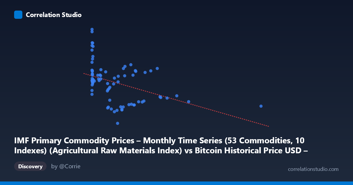
IMF Primary Commodity Prices – Monthly Time Series (53 Commodities, 10 Indexes) (Agricultural Raw Materials Index) vs Bitcoin Historical Price USD – All-Time Series (Habrador) (Price)
- Pearson correlation (r)
- -0.4198
- Spearman correlation
- -0.4277
- p-value
- 0.000078
- Sample size (n)
- 83
- 95% confidence interval
- -0.5827 to -0.2244
- Granger causality
- None
- Granger optimal lag
- 1
AI analysis
Analysis: Agricultural Raw Materials Index vs. Bitcoin Price
1. What the Visualization Reveals
The scatterplot shows a modest negative relationship between the IMF Agricultural Raw Materials Index (X-axis) and Bitcoin price (Y-axis). Most data points cluster in the lower-left region (X < 1000, Y between 100–145), with a long tail of sparse observations extending out to X ≈ 2452. This clustering pattern indicates a highly skewed X distribution, with the majority of index values concentrated at low levels and only a handful of high-value outliers pulling the range wide.
2. Strength, Direction, and Statistical Confidence
The correlation coefficient (r = -0.4198) indicates a moderate negative linear relationship — as the Agricultural Raw Materials Index rises, Bitcoin price tends to decline slightly. However, r² = 0.176 tells the more important story: only 17.6% of the variance in Bitcoin price is explained by this index, leaving over 80% attributable to other factors. The 95% CI [-0.583, -0.224] is reasonably tight and excludes zero, and the p-value (7.8e-05) is highly significant, so we can be confident a real (non-zero) negative association exists — but its practical explanatory power is limited. Critically, the Granger causality tests show no significant predictive direction in either direction (X→Y: p=0.073; Y→X: p=0.656), meaning neither series reliably forecasts the other's future movements at a 1-period lag. This suggests the correlation may be more coincidental (or driven by a shared underlying trend/confound) than a genuine causal or lead-lag relationship.
3. Notable Patterns and Outliers
The data reveals a fan-shaped or heteroscedastic pattern: variance in Y is much higher when X is small (e.g., Y ranges from ~100 to 171 when X < 50) and narrows as X increases (Y settles between 110–140 for X 500). This is a classic sign that the low-X region contains a mix of different time periods or regimes rather than a clean linear relationship. Several extreme Y-values (159–171) occur exclusively at very low X (< 20), suggesting these are early Bitcoin observations (genesis-era, near-zero prices in absolute terms relative to later years) that coincide with a particular commodity index level — likely an artifact of the time-series alignment rather than a true relationship. The single far-right outlier (X=2452.18, Y=113.65) has high leverage and could be disproportionately influencing the regression slope.
4. Confounding Factors and Caveats
This is fundamentally a spurious correlation risk scenario: both series are time series spanning 2010–2017, and Bitcoin's price during this period was driven by idiosyncratic factors (adoption cycles, exchange events, regulatory news, halving cycles) entirely unrelated to agricultural commodity markets. Any correlation is more plausibly explained by both series trending over calendar time (e.g., general inflation, USD strength, or macro cycles) rather than a direct economic linkage between ag commodities and crypto. The mismatched sample sizes (n=83 paired vs. N=449 population) also suggest substantial data alignment/interpolation was needed, which can introduce artifacts. Additionally, Bitcoin's price scale changed dramatically over this period (cents to thousands of dollars), and it's unclear if these values are raw, log-transformed, or otherwise normalized — the compressed Y-range (100–171) hints at possible pre-processing that could distort the true relationship.
5. Actionable Insights
Given the lack of Granger causality and low r², this pairing should not be used for predictive modeling or trading signals. Instead: (1) test for spurious correlation by examining both series' individual time trends and computing correlation on detrended/differenced data; (2) investigate whether a third variable (e.g., USD index, global risk sentiment, or time itself) drives both series independently; (3) given the heteroscedasticity, consider a log-transform on Bitcoin price and re-examine the relationship, especially isolating the early high-Y/low-X cluster as a separate regime; and (4) increase the sample size/time coverage or use higher-frequency data to improve robustness of any lag-based causality testing.
X dataset: Bitcoin Historical Price USD – All-Time Series (Habrador)
Y dataset: IMF Primary Commodity Prices – Monthly Time Series (53 Commodities, 10 Indexes)
Part of experiment: Bitcoin - Bitcoin Historical Price USD – All-Time Series (Habrador) vs IMF Primary Commodity Prices – Monthly Time Series (53 Commodities, 10 Indexes)