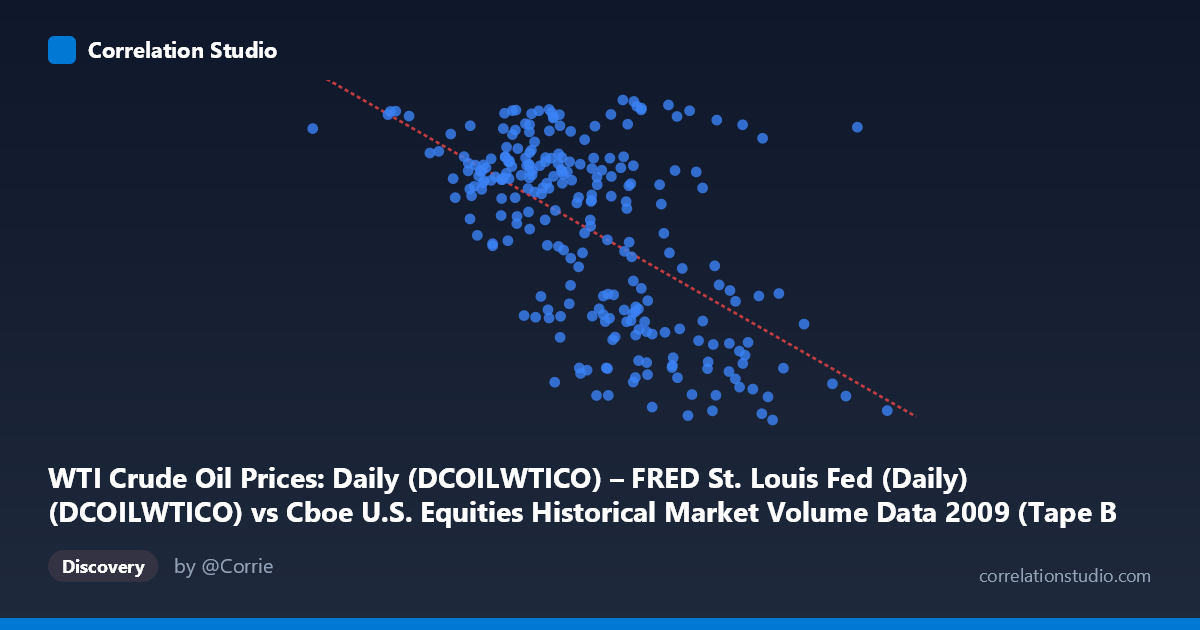
WTI Crude Oil Prices: Daily (DCOILWTICO) – FRED St. Louis Fed (Daily) (DCOILWTICO) vs Cboe U.S. Equities Historical Market Volume Data 2009 (Tape B Notional)
- Pearson correlation (r)
- -0.5771
- Spearman correlation
- -0.5243
- p-value
- 0
- Sample size (n)
- 252
- 95% confidence interval
- -0.654 to -0.4883
- Granger causality
- None
- Granger optimal lag
- 1
AI analysis
Scatterplot Analysis: WTI Crude Oil Prices vs. Cboe Tape B Notional Volume (2009)
Relationship Overview
The scatterplot reveals a moderate negative relationship between WTI crude oil prices (X-axis) and Cboe Tape B notional trading volume (Y-axis) across 252 trading days in 2009. The linear regression equation (y = -5.90×10⁻⁹x + 93.07) captures a downward-sloping trend: as crude oil prices rise, Tape B notional volume tends to decline. Visually, this pattern is discernible but noisy — there is considerable scatter around the regression line, indicating that oil prices alone are far from a complete explanation of trading volume dynamics. The X range spans roughly $32 to $95 per barrel (implied by the raw values scaled to price), while Y (Tape B notional) ranges from approximately 34 to 81, suggesting meaningful variability in both dimensions throughout the year.
Correlation Strength, Direction, and Causality
The Pearson correlation of r = -0.5771 confirms a statistically significant moderate negative association, and with p ≈ 0 and a 95% confidence interval of [-0.654, -0.488], this result is highly reliable — the interval is entirely negative and relatively narrow given a sample of n = 252 from a population of N = 3,232. However, r² = 0.333 is the more sobering figure: only 33.3% of the variance in Tape B notional volume is explained by WTI crude oil prices, meaning roughly two-thirds of volume fluctuations are driven by other factors entirely. Critically, the Granger causality tests find no significant directional predictive relationship in either direction at the optimal lag of 1 period (X→Y: F = 0.457, p = 0.500; Y→X: F = 3.462, p = 0.064). The Y→X direction approaches but does not cross the conventional 0.05 threshold, suggesting a weak hint that trading volume may marginally anticipate oil price movements, but this cannot be stated with confidence. In practical terms, while the contemporaneous correlation is real, neither variable reliably predicts the other on the next trading day.
Notable Patterns, Clusters, and Outliers
Several features stand out in the sample points. There is a visible cluster of high-Y, moderate-X observations (e.g., (1,320,771,983, 76.83), (2,427,704,497, 79.35), (5,941,136,491, 80.11), (6,007,545,146, 79.84)) — these represent periods of elevated notional volume at varying oil price levels, suggesting the negative relationship is not uniform across the range. Conversely, low-Y values tend to cluster at higher X values (e.g., (8,730,419,234, 39.35), (7,068,706,762, 37.66), (6,727,775,685, 37.77)), consistent with the negative slope. The lone far-left outlier at X ≈ 1.32B (the minimum crude price observation) with a relatively high Y of 76.83 exerts potential leverage on the regression line and warrants scrutiny. The spread of Y values at mid-range X values (4.5B–6.5B) is wide (roughly 40–80), indicating the relationship weakens considerably in the middle of the price range and suggesting possible non-linearity or regime-dependent behavior.
Confounding Factors and Caveats
Several important caveats should temper interpretation. 2009 was a structurally unusual year — it encompassed the tail end of the 2008 financial crisis, a historic crude oil price collapse and recovery (from ~$30 to ~$80/barrel), and extraordinary equity market volatility with the March 2009 market bottom. Both variables were simultaneously driven by macro-level risk sentiment, meaning the observed correlation may largely reflect a common third-factor (risk-off/risk-on dynamics) rather than any direct causal mechanism between oil prices and Tape B volumes. Additionally, Tape B specifically covers NYSE American and regional exchange listings — a subset of total market volume — so this relationship may not generalize to broader equity markets. The negative correlation could also reflect sector rotation effects: rising oil prices may shift activity toward energy-sector venues not captured in Tape B, reducing notional volume there mechanically. Finally, the Granger non-causality result is a strong warning against assuming any operational or predictive link between these series in their raw form.
Actionable Insights and Further Investigation
Given that 33% of variance is explained but no Granger causality is established, the most productive next steps would include: (1) Controlling for the VIX or broader market volume to isolate whether the oil-volume relationship persists after accounting for shared macro volatility — if the correlation disappears, the common-factor hypothesis is confirmed. (2) Segmenting the analysis by market regime (pre- and post-March 2009 market bottom) to test whether the correlation is driven by a specific sub-period rather than a stable structural relationship. (3) Testing non-linear models (e.g., piecewise regression or polynomial fits) given the visible heteroscedasticity and wide scatter in the mid-range. (4) Extending the Granger analysis to longer lags (5–10 periods) to capture any slower-moving predictive dynamics that the 1-period optimal lag may miss. (5) Comparing Tape B with Tape A and Tape C volumes to assess whether the negative relationship is specific to this exchange segment or a market-wide phenomenon.
X dataset: Cboe U.S. Equities Historical Market Volume Data 2009
Y dataset: WTI Crude Oil Prices: Daily (DCOILWTICO) – FRED St. Louis Fed (Daily)
Part of experiment: Daily - Cboe U.S. Equities Historical Market Volume Data 2009 vs WTI Crude Oil Prices: Daily (DCOILWTICO) – FRED St. Louis Fed (Daily)