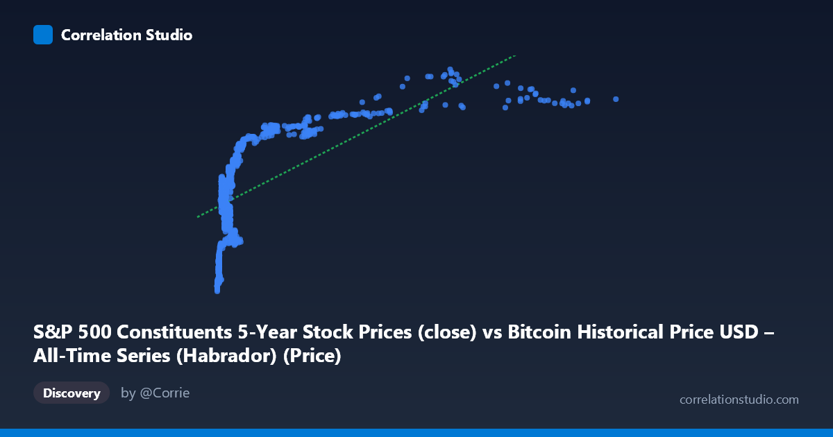
S&P 500 Constituents 5-Year Stock Prices (close) vs Bitcoin Historical Price USD – All-Time Series (Habrador) (Price)

Pearson correlation (r): 0.6348
Spearman correlation: 0.7164
p-value: 0
Sample size (n): 1259
95% confidence interval: 0.6006 to 0.6667
Granger causality: X → Y
Granger optimal lag: 1
Time coverage: 2013-02-08 to 2018-02-07

AI analysis

Analysis: Bitcoin Price vs. S&P 500 Constituent Prices

1. Relationship Overview

The scatterplot depicts a positive, moderately strong association between Bitcoin's historical USD price (X) and an aggregated measure of S&P 500 constituent stock prices (Y). The data shows a clear non-linear/logarithmic-like pattern: Y rises steeply as X moves from near-zero to a few thousand dollars, then the rate of increase flattens as X grows into the tens of thousands. This is typical of variables where one spans several orders of magnitude (X ranges from ~23 to ~18,960) while the other is comparatively compressed (Y ranges from 57 to 115).

2. Strength, Direction, and Statistical Confidence

The correlation coefficient (r = 0.635) indicates a moderate positive linear relationship, with r² = 0.403 meaning only about 40% of the variance in Y is explained by X — leaving the majority (60%) attributable to other factors or non-linear dynamics not captured by this simple linear fit. The 95% CI [0.601, 0.667] is fairly tight given the large sample (n = 1,259), and the p-value of ~0 confirms the correlation is statistically significant and not due to chance. However, statistical significance here reflects the large sample size more than practical predictive strength — r² of 0.40 leaves considerable unexplained variance for any real-world forecasting use.

The Granger causality results add a temporal dimension: X (Bitcoin) Granger-causes Y (S&P prices) at lag 1 (F = 4.86, p = 0.028), while the reverse (Y→X) is not significant (p = 0.62). This suggests Bitcoin price movements have modest predictive power for subsequent S&P price movements, but not vice versa — an asymmetric, unidirectional temporal relationship rather than true bidirectional causation.

3. Notable Patterns and Features

The clustering of points reveals distinct regimes: a dense cluster of low-X, low-to-mid-Y values (X < 1,000, Y in 60-90 range) corresponding to Bitcoin's early years, and a sparser set of high-X points (X 6,000) all clustering near Y = 100-115, corresponding to Bitcoin's 2017 bull run. This creates a curved, saturating shape rather than a straight line — the relationship resembles a logarithmic or power curve better than linear, which likely explains why r² caps at ~40%. There's also noticeable vertical scatter at low X values (e.g., X≈580-650 producing Y from 75 to 89), indicating substantial noise or additional drivers at that range.

4. Confounding Factors and Caveats

This is a critical caveat: both series are time series with strong trends, and the "correlation" is very likely driven by mutual trending over the 2013–2018 window rather than genuine economic linkage. Bitcoin and S&P 500 stocks were both in prolonged bull markets during this period for largely independent reasons (crypto speculation vs. post-financial-crisis equity recovery, low rates, tech growth). This is a classic case of spurious correlation via co-trending non-stationary series — the Granger test on raw (likely non-stationary) price levels can produce misleading significance; results should be re-run on differenced/returns data to check robustness. Additionally, "S&P 500 constituent prices" as a single column is ambiguous (average? single stock? index proxy?), which complicates economic interpretation.

5. Suggestions for Further Investigation

1. Detrend/difference the data — re-run correlation and Granger tests on daily/weekly returns rather than price levels to test whether the relationship survives after removing shared trend components. 2. Test log-transforms — given Bitcoin's exponential growth, regressing log(X) or log(Y) against the other may yield a better-fitting, more interpretable model than the linear fit (R²=0.403). 3. Control for time/macro factors — include a time trend or macro variables (interest rates, USD index) to check if the X→Y Granger result survives, distinguishing genuine lead-lag dynamics from common drivers. 4. Segment by regime — analyze the pre-2017 vs. 2017 bull-run periods separately, since pooling regimes may be inflating or distorting the overall r².

X dataset: Bitcoin Historical Price USD – All-Time Series (Habrador)

Y dataset: S&P 500 Constituents 5-Year Stock Prices

Part of experiment: Bitcoin - Bitcoin Historical Price USD – All-Time Series (Habrador) vs S&P 500 Constituents 5-Year Stock Prices