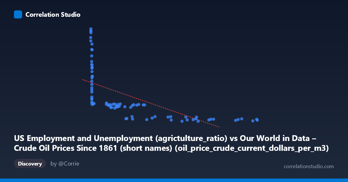
US Employment and Unemployment (agrictulture_ratio) vs Our World in Data – Crude Oil Prices Since 1861 (short names) (oil_price_crude_current_dollars_per_m3)
- Pearson correlation (r)
- -0.6372
- Spearman correlation
- -0.9155
- p-value
- 0
- Sample size (n)
- 85
- 95% confidence interval
- -0.7486 to -0.4907
- Granger causality
- None
- Granger optimal lag
- 10
AI analysis
Analysis of US Agriculture Employment Ratio vs. Crude Oil Prices
1. Overall Relationship Pattern
The scatterplot reveals a negative relationship between the US agriculture employment ratio (X) and crude oil prices in current dollars per cubic meter (Y). The data spans from 1941 to 2024, capturing major structural shifts in both the US labor market and global energy markets. Visually, the pattern is notably non-linear: when the agriculture ratio is very low (roughly below 20–30), oil prices span an exceptionally wide range — from under 3,000 to over 9,000 — while at higher agriculture ratios (above ~70), oil prices cluster tightly in a narrow band around 2,100–3,500. This funnel-shaped or hyperbolic dispersion strongly suggests a logarithmic or power relationship rather than a simple linear one, which is confirmed by the note that Spearman ρ exceeds Pearson r.
2. Correlation Strength, Direction, and Causality
The Pearson correlation of r = −0.6326 indicates a moderate-to-strong negative association: as the share of employment in agriculture declines, crude oil prices tend to rise. However, framing this through r² = 0.4001 is essential — only 40% of the variance in oil prices is explained by the agriculture employment ratio, meaning 60% of oil price variation is driven by other factors entirely. The 95% confidence interval of [−0.7458, −0.4838] is comfortably away from zero, and the p-value of 1.085 × 10⁻¹⁰ confirms this correlation is highly statistically significant — not a chance finding across 84 paired observations. Despite this statistical significance, Granger causality tests find no significant predictive direction in either direction (X→Y: F = 1.18, p = 0.32; Y→X: F = 1.41, p = 0.20 at optimal lag 10). This is a critical qualifier: the correlation, while real, does not imply that changes in the agriculture employment ratio temporally precede and predict changes in oil prices, nor vice versa. Both variables appear to be co-evolving with time — likely driven by shared underlying trends — rather than one causing the other.
3. Notable Patterns, Clusters, and Outliers
The data separates into two visually distinct behavioral regimes. The first cluster sits at high agriculture ratios (roughly X = 60–350) with oil prices compressed between ~2,100 and ~3,500 — this almost certainly corresponds to the mid-20th century era (1940s–1970s) when US farm employment was still substantial and oil was cheap in real terms. The second and more dramatic cluster occupies the low agriculture-ratio zone (X < 20), where oil prices are highly variable and elevated, spanning 2,095 to 9,250 — reflecting the post-1980s and 2000s era of near-complete agricultural mechanization alongside volatile global oil markets. Several clear outliers appear at very low X values (6.6–15) with extremely high Y values (7,629–9,250), likely corresponding to oil price spikes around 2008, 2011–2014, or 2022. These high-leverage points substantially influence the regression slope and correlation coefficient.
4. Confounding Factors and Interpretive Caveats
The most significant caveat is that both variables are proxies for the passage of time and broader economic modernization rather than causally linked phenomena. The agriculture employment ratio has declined monotonically across the 20th century due to mechanization, urbanization, and structural economic change — entirely independent of oil markets. Oil prices, meanwhile, reflect geopolitical events (OPEC embargoes, Gulf Wars, COVID demand collapse), technological changes in extraction (shale revolution), and global demand growth from industrializing nations. The shared time trend creates a spurious or confounded correlation: both happened to move together because both are products of the same era of industrialization. The linear regression (y = −6.43x + 5,147) also likely understates the relationship at low agriculture ratios and overstates it at high ones, given the non-linear dispersion pattern observed.
5. Actionable Insights and Further Investigation
Given the evidence of non-linearity, the immediate analytical recommendation is to refit using a logarithmic or inverse model (e.g., y = a·ln(x) + b or y = a/x + b), which would likely improve the explained variance beyond the current 40% and better capture the hyperbolic dispersion. More importantly, detrending both series (e.g., removing the shared time trend via first-differencing or regression on year) before computing correlation would test whether any genuine relationship exists beyond the common temporal trend — this is arguably the most important next step. Researchers should also consider inflation-adjusting oil prices to separate real price changes from nominal drift. Finally, the Granger non-causality finding strongly suggests that multivariate models incorporating explicit time controls, energy policy variables, and GDP would be more informative than this bivariate analysis alone for understanding what actually drives crude oil price variation over this historical period.
X dataset: Our World in Data – Crude Oil Prices Since 1861 (short names)
Y dataset: US Employment and Unemployment
Part of experiment: Yearly - Our World in Data – Crude Oil Prices Since 1861 (short names) vs US Employment and Unemployment