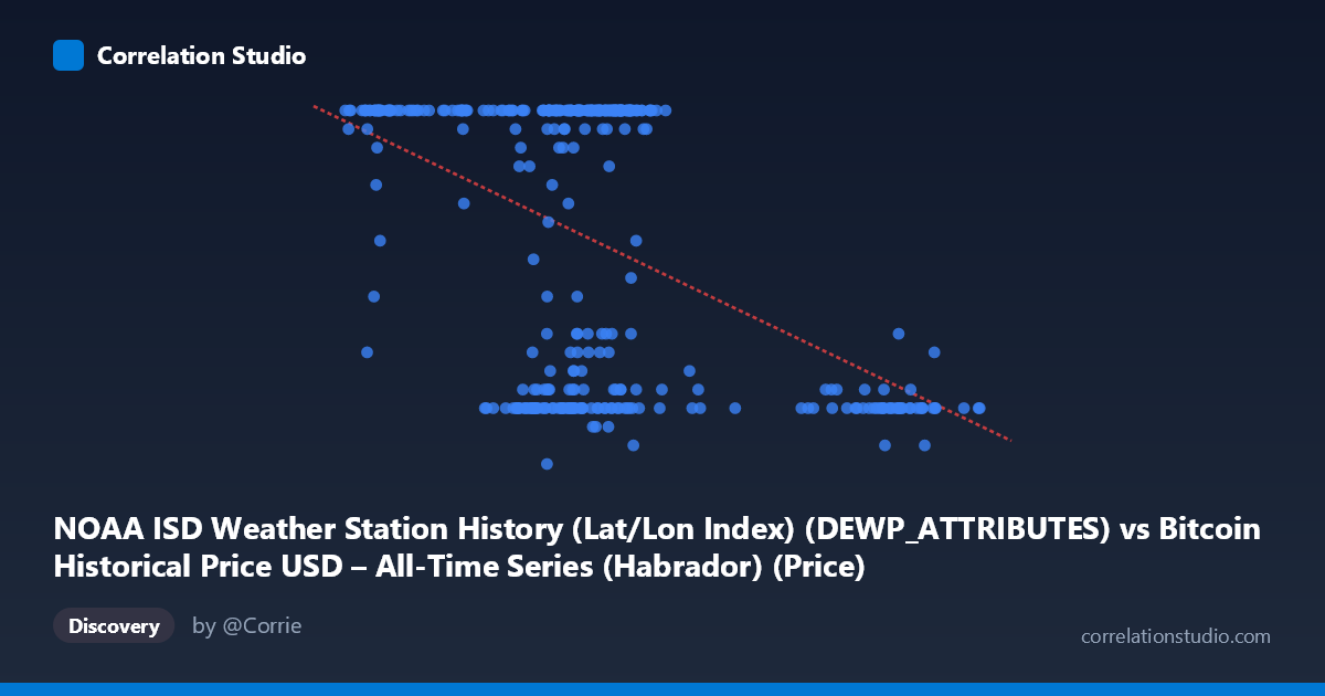
NOAA ISD Weather Station History (Lat/Lon Index) (DEWP_ATTRIBUTES) vs Bitcoin Historical Price USD – All-Time Series (Habrador) (Price)
- Pearson correlation (r)
- -0.4722
- Spearman correlation
- -0.3069
- p-value
- 0
- Sample size (n)
- 355
- 95% confidence interval
- -0.5493 to -0.3871
- Granger causality
- None
- Granger optimal lag
- 1
AI analysis
Analysis of Correlation Between Variables
1. Overview of the Relationship
The scatterplot displays a moderate negative relationship between the two variables (labeled as DEWPATTRIBUTES on X and Price on Y, though these labels appear to be mismatched/misassigned given the dataset descriptions reference Bitcoin price history and NOAA weather station data). The data shows a downward-sloping pattern, with the regression line (y = -0.000246x + 33.13) confirming that as X increases, Y tends to decrease. However, the scatter is substantial, indicating this is a loose statistical association rather than a tight deterministic relationship.
2. Strength, Direction, and Statistical Confidence
The correlation coefficient of r = -0.4722 indicates a moderate negative linear relationship. Critically, r² = 0.2229 means only about 22% of the variance in Y is explained by X — the remaining 78% is driven by other factors, noise, or non-linear dynamics not captured by this simple linear model. Despite this modest explanatory power, the relationship is statistically robust: the 95% confidence interval [-0.5493, -0.3871] is narrow and entirely negative, and the p-value of 0 (effectively p < 0.001) confirms this correlation is highly unlikely to be due to chance, especially with n=355 paired observations. That said, statistical significance should not be conflated with practical strength — this is a real but weak-to-moderate effect. The Granger causality tests further temper any causal interpretation: neither direction shows significant predictive power (X→Y: p=0.58; Y→X: p=0.27), meaning neither variable helps forecast the other over time. This strongly suggests the correlation reflects a contemporaneous or coincidental association rather than a lagged causal mechanism.
3. Notable Patterns and Outliers
The sample data reveals an interesting structural feature: Y values cluster heavily at specific levels — particularly 24 (appearing extremely frequently) and a lower cluster around 8-12. This bimodal/discretized clustering suggests Y may be a bounded, categorical, or capped variable (e.g., possibly representing a count, rating, or capped measurement) rather than a smooth continuous variable. Looking at X, most values cluster between 41,000-72,000, with several outliers extending to 90,000-106,000 — and notably, these higher-X outliers consistently pair with lower Y values (8-11), which likely drives much of the negative correlation. This pattern suggests the relationship may be driven by a subset of extreme X values rather than a uniform linear trend across the full range.
4. Confounding Factors and Caveats
Several caveats warrant attention. First, the axis labels appear inconsistent with the dataset descriptions (Bitcoin price vs. NOAA weather attributes swapped), suggesting a possible data pipeline or labeling error that should be verified before drawing substantive conclusions. Second, the apparent capping/clustering of Y at 24 (and the lower cluster near 8-9) suggests measurement truncation, categorical encoding, or a ceiling effect — this could artificially inflate or distort the correlation coefficient. Third, both series may be independently trending over time (2024 full-year coverage), raising the risk of spurious correlation via shared temporal trends rather than genuine interaction — a common issue when combining financial time series (Bitcoin price) with unrelated environmental data (weather stations). Finally, the outlier cluster at high X values (90k-106k) has disproportionate leverage on the regression slope.
5. Recommendations for Further Investigation
1. Verify data labeling/pairing — confirm the X and Y columns are correctly assigned and that pairing Bitcoin price with a specific weather station's dew point attributes is intentional and meaningful. 2. Investigate the Y-variable clustering — determine why values concentrate at 24 and 8-9; consider whether Y should be treated as ordinal/categorical rather than continuous. 3. Test for non-linearity — given low r² and visible clustering, explore piecewise, logistic, or quantile regression models. 4. Detrend both series — since Granger causality is absent, check whether correlation is spurious due to shared annual trends (e.g., both varying by season/month independently). 5. Isolate outliers — re-run correlation excluding the high-X cluster (90k+) to see if the relationship holds in the core data range or is outlier-driven.
X dataset: Bitcoin Historical Price USD – All-Time Series (Habrador)
Y dataset: NOAA ISD Weather Station History (Lat/Lon Index)
Part of experiment: Bitcoin - Bitcoin Historical Price USD – All-Time Series (Habrador) vs NOAA ISD Weather Station History (Lat/Lon Index)