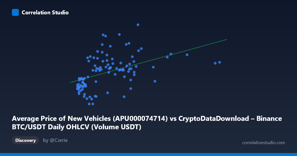
Average Price of New Vehicles (APU000074714) vs CryptoDataDownload – Binance BTC/USDT Daily OHLCV (Volume USDT)
- Pearson correlation (r)
- 0.4686
- Spearman correlation
- 0.5955
- p-value
- 0
- Sample size (n)
- 106
- 95% confidence interval
- 0.3051 to 0.6052
- Granger causality
- None
- Granger optimal lag
- 1
- Time coverage
- 2017-09-01 to 2026-06-01
- Recomputed on refreshed data
- 2026-10-21 (r was 0.4686)
AI analysis
Analysis: BTC/USDT Trading Volume vs. Average New Vehicle Prices
1. Overview of the Relationship
The scatterplot displays a positive but moderate association between two variables that, notably, appear to be mislabeled or swapped in the metadata — the X-axis values (ranging into the billions) align with "Volume USDT" behavior, while the Y-axis (1.88–5.06) looks more like a normalized or transformed price index rather than raw vehicle prices. Regardless of labeling, the pattern shows that as X increases, Y tends to increase as well, though with substantial scatter around the trend line, indicating a loose rather than tight coupling.
2. Strength, Direction, and Statistical Confidence
The Pearson correlation of r = 0.489 indicates a moderate positive relationship, but r² = 0.239 reveals that only about 24% of the variance in Y is explained by X — meaning roughly three-quarters of Y's variability is driven by other factors entirely. The 95% CI [0.327, 0.623] is reasonably tight and excludes zero, and the p-value (1.39E-07) confirms this correlation is highly statistically significant and not a product of chance, even though it's a modest effect size in practical terms. Critically, the Granger causality tests show no significant predictive direction in either direction (X→Y: p=0.395; Y→X: p=0.836). This means that despite the contemporaneous correlation, past values of one series do not meaningfully help forecast future values of the other — the relationship, if real, is not a simple lead-lag dynamic and may instead reflect a shared external driver or coincidental co-trending over the 2017–2026 window.
3. Notable Patterns and Features
The data shows a wide spread at low-to-mid X values (roughly under 1 billion), with Y ranging anywhere from ~1.88 to ~3.9, suggesting high noise in this region. At higher X values (above 2 billion), Y values cluster more tightly in the 3.0–4.7 range, hinting at a possible threshold or saturation effect rather than a strictly linear relationship. The note that Spearman ρ exceeds Pearson r is important — it suggests the true relationship may be monotonic but non-linear (e.g., logarithmic or power-law), which is common when one variable spans several orders of magnitude (as X does here, from ~2.6M to ~7.4B). A log-transformation of X would likely produce a cleaner, more linear fit and a higher explained variance.
4. Confounding Factors and Caveats
Given the described datasets (crypto trading volume and vehicle price inflation), any correlation is almost certainly spurious or mediated by a common macro trend — both cryptocurrency markets and vehicle prices have been influenced by broad inflationary pressure, pandemic-era supply chain disruptions, and loose monetary policy from 2020–2022, which could create a false sense of direct relationship. Time-series data like this is also prone to autocorrelation and trending, which inflates correlation coefficients even when no causal link exists. The mismatched axis labels/units raise a data-integrity concern that should be resolved before drawing further conclusions. Additionally, with n=104 paired points drawn from a larger population of 604, sampling/aggregation choices (e.g., which dates were matched between daily crypto data and monthly vehicle data) could introduce artifacts.
5. Recommendations
Before treating this as a meaningful relationship, verify and correct the axis/column labeling to ensure X and Y correspond to their intended datasets. Next, test a log-linear or log-log model given the extreme right-skew in X and the Spearman/Pearson discrepancy — this will likely improve fit and clarify whether the relationship is truly monotonic. Since Granger causality is absent, avoid using one series to forecast the other in any trading or economic model; instead, investigate shared confounders (e.g., CPI, USD strength, or a common macro index) using multivariate regression or a third-variable control. Finally, given the mixed frequency (daily crypto vs. monthly vehicle prices), consider resampling to a consistent time granularity to reduce noise from misaligned observations.
X dataset: CryptoDataDownload – Binance BTC/USDT Daily OHLCV
Y dataset: Average Price of New Vehicles
Part of experiment: Bitcoin - CryptoDataDownload – Binance BTC/USDT Daily OHLCV vs Average Price of New Vehicles