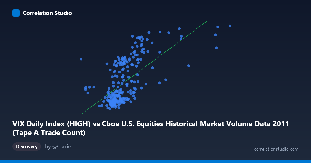
VIX Daily Index (HIGH) vs Cboe U.S. Equities Historical Market Volume Data 2011 (Tape A Trade Count)
- Pearson correlation (r)
- 0.6497
- Spearman correlation
- 0.6749
- p-value
- 0
- Sample size (n)
- 252
- 95% confidence interval
- 0.572 to 0.7158
- Granger causality
- None
- Granger optimal lag
- 1
AI analysis
Scatterplot Analysis: VIX High vs. Tape A Trade Count (2011)
Overall Relationship The scatterplot reveals a moderately strong positive relationship between the VIX Daily Index High values and Cboe U.S. Equities Tape A Trade Count during 2011. As VIX High values increase, trade counts tend to rise correspondingly, which is intuitively consistent with the well-established market behavior that heightened volatility drives increased trading activity. The linear regression equation (y = 1.806×10⁻⁵x + 3.807) confirms this upward slope, and the visual pattern shows a reasonably coherent trend despite considerable scatter, particularly at higher VIX levels.
Correlation Strength and Statistical Significance The Pearson correlation of r = 0.6497 indicates a moderate-to-strong positive association. However, the r² of 0.4221 is the more telling statistic — it means that approximately 42.2% of the variance in Tape A Trade Count is explained by VIX High, leaving roughly 57.8% attributable to other factors. The 95% confidence interval for r [0.5720, 0.7158] is meaningfully narrow given n = 252, and the p-value of effectively zero confirms this relationship is not a chance artifact in the sample. That said, the Granger causality tests reveal no statistically significant temporal predictive direction in either direction (X→Y: F = 0.228, p = 0.633; Y→X: F = 0.094, p = 0.760). This is a critical caveat: while the contemporaneous correlation is robust, neither variable reliably predicts the other with a one-period lag, suggesting the relationship is largely coincident rather than directionally causal at the daily frequency examined.
Notable Patterns, Clusters, and Outliers Several structural features stand out in the data: - A dense lower cluster is visible roughly in the X range of 900,000–1,300,000 with Y values below ~25, suggesting a large base of "normal" low-volatility trading days concentrated in this zone. - A dispersed upper arm extends toward higher X and Y values, with notable spread — points like (1,453,966, 42.99), (1,487,505, 42.00), (2,126,542, 42.88), and (1,519,331, 38.74) represent elevated trade count days coinciding with high VIX periods. - The point at approximately (2,126,542, 42.88) appears to be a potential high-leverage outlier — the X value is nearly twice the mean and substantially beyond the next-highest observations, likely corresponding to a peak volatility event in 2011 (possibly the August U.S. debt ceiling crisis or European sovereign debt escalation). - The relationship also shows heteroscedasticity: variance in trade counts visibly fans out at higher VIX levels, suggesting the linear model understates uncertainty during volatile regimes.
Confounding Factors and Caveats Several important confounders should temper interpretation. First, 2011 was an atypically volatile year — the U.S. credit downgrade and European debt crisis created extreme observations that may be disproportionately driving the correlation; the relationship may look quite different in calmer years. Second, secular trends in trading volume (e.g., algorithmic trading growth, exchange competition) could create spurious correlation if both variables trended similarly over time independent of each other. Third, the axes appear swapped from conventional expectation — VIX is plotted on X and trade count on Y, but the dataset metadata suggests the column labels may be cross-assigned between datasets, warranting verification of which series is truly which. Finally, the Granger non-result at lag-1 may simply reflect that a one-day lag is too coarse or that the relationship operates within-day rather than day-to-day.
Actionable Insights and Further Investigation Practitioners should consider the following steps: (1) Test multiple Granger lags (e.g., 2–5 days) and intraday frequencies to better characterize the temporal dynamics; (2) Segment the analysis by volatility regime (e.g., VIX < 20 vs. ≥ 20) to test whether the relationship is driven primarily by tail events; (3) Include additional predictors such as market returns, news sentiment, or options expiration calendars to build a more complete model of trade count variance; (4) Replicate across multiple years to assess whether this correlation is stable or specific to 2011's extraordinary macro environment; and (5) Address the heteroscedasticity with log-transformation of trade counts or a robust regression approach, which may improve both model fit and interpretability at extreme VIX levels.
X dataset: Cboe U.S. Equities Historical Market Volume Data 2011
Y dataset: VIX Daily Index
Part of experiment: Daily - Cboe U.S. Equities Historical Market Volume Data 2011 vs VIX Daily Index