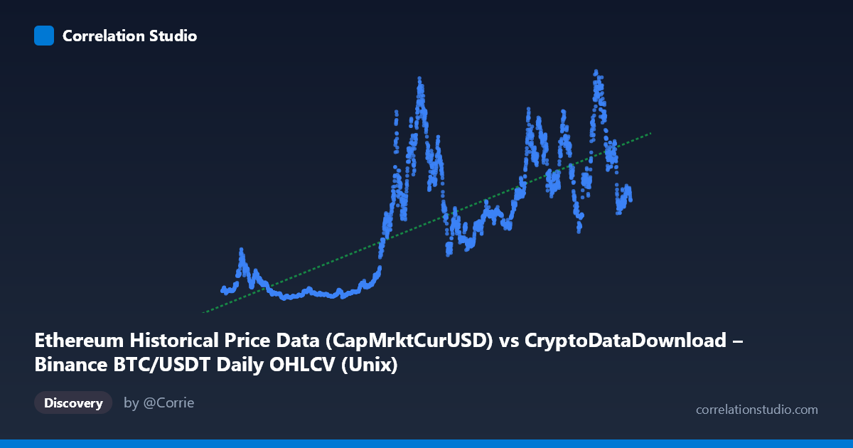
Ethereum Historical Price Data (CapMrktCurUSD) vs CryptoDataDownload – Binance BTC/USDT Daily OHLCV (Unix)
- Pearson correlation (r)
- 0.7712
- Spearman correlation
- 0.7664
- p-value
- 0
- Sample size (n)
- 3191
- 95% confidence interval
- 0.7567 to 0.7849
- Granger causality
- X → Y
- Granger optimal lag
- 10
AI analysis
Analysis: Time (X) vs. Ethereum/Bitcoin Market Metric (Y)
1. What the Visualization Reveals
The scatterplot shows a time-series variable (X, labeled as a timestamp field but functioning here as a date axis spanning August 2017 to May 2026) plotted against a monetary/market-cap-style metric (Y, ranging from ~$8.6B to ~$584B). Rather than a classical bivariate relationship between two independent measures, this is effectively Y plotted against time, meaning the "correlation" is really describing a long-term growth trend with substantial cyclical volatility layered on top. The data shows Y climbing from tens of billions in 2017-2020 to peaks exceeding $400-500B in 2021-2022 and again in 2024-2025, consistent with known Bitcoin/Ethereum market cycles.
2. Strength, Direction, and Statistical Confidence
The correlation coefficient (r = 0.771, r² = 0.595) indicates a moderately strong positive relationship, but with an important caveat: only 59.5% of the variance in Y is explained by X (time). The remaining ~40% is driven by other factors — likely market cycles, halving events, macro liquidity conditions, and speculative sentiment — not captured by a simple linear time trend. The 95% CI [0.757, 0.785] is tight given the large sample (n=3,191), and p≈0 confirms the relationship is highly statistically significant and not due to chance. However, statistical significance here reflects the strong autocorrelation inherent in time-series data rather than a meaningful causal driver.
The Granger causality result (X→Y significant at F=1.85, p=0.048; Y→X not significant, p=0.695) suggests a weak but detectable unidirectional predictive relationship from X to Y at a 10-period lag. Given X is essentially a time index, this result is somewhat tautological — it mainly confirms that past values of the price series help predict future values (i.e., Y has momentum/trend-following behavior), not that "time" is a causal driver in an economically meaningful sense.
3. Notable Patterns and Non-linearities
The linear fit (y = 1.504x − 2.269e12, R²=0.595) is a poor descriptor of the actual dynamics. The data clearly exhibits: - Cyclical boom-bust structure: sharp run-ups (2020-2021, 2023-2024) followed by drawdowns, rather than monotonic growth. - Heteroscedasticity: variance in Y increases substantially in later periods — early data clusters tightly near $15-70B, while later data ranges widely from $150B to $580B. - Multiple regimes/clusters: at least two or three distinct "plateau" clusters are visible (2017-2020 lower band, 2021-2022 middle band, 2024-2025 upper band), suggesting regime shifts rather than a single smooth trend. - A linear model will systematically underpredict during bull peaks and overpredict during bear troughs.
4. Confounding Factors and Caveats
Several caveats limit interpretation: - Spurious time-trend correlation: Any monotonically growing series (adoption, market cap, users) will show high r² against time without implying meaningful causality. - Non-stationarity: Both series likely have unit-root/trending behavior, inflating correlation and Granger test statistics (spurious regression risk). Differencing or detrending is needed before trusting the Granger results. - Cross-dataset mismatch: The X and Y labels reference two different datasets (BTC/USDT OHLCV vs. Ethereum network metrics), raising questions about whether the "correlation" reflects genuine BTC-ETH co-movement or an artifact of merging/aligning timestamps. - Autocorrelation inflates significance: Daily granularity with strong serial correlation means effective sample size is much smaller than n=3,191, making the p-values overly optimistic.
5. Suggested Next Steps
- De-trend or difference both series (e.g., use log returns or % changes) and re-run correlation/Granger tests to check if the relationship holds after removing shared trend/non-stationarity. - Segment by market regime (bull/bear/consolidation) to see if the X-Y relationship is stable or regime-dependent. - Test BTC price vs. ETH market cap directly (rather than vs. time) to assess genuine cross-asset correlation, which is likely the more economically interesting relationship. - Use rolling-window correlation to visualize how the relationship strength changes over the 2017-2026 period, since a single r value likely masks significant time-varying dynamics.
X dataset: CryptoDataDownload – Binance BTC/USDT Daily OHLCV
Y dataset: Ethereum Historical Price Data
Part of experiment: Bitcoin - CryptoDataDownload – Binance BTC/USDT Daily OHLCV vs Ethereum Historical Price Data