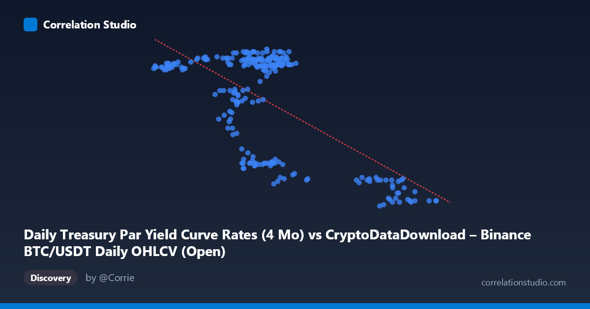
Daily Treasury Par Yield Curve Rates (4 Mo) vs CryptoDataDownload – Binance BTC/USDT Daily OHLCV (Open)
- Pearson correlation (r)
- -0.6564
- Spearman correlation
- -0.3327
- p-value
- 0
- Sample size (n)
- 250
- 95% confidence interval
- -0.7217 to -0.5795
- Granger causality
- None
- Granger optimal lag
- 1
- Time coverage
- 2024-01-02 to 2024-12-31
AI analysis
Analysis of Treasury Yield vs. Treasury Par Yield Rate Relationship
Note on axis labeling: The provided axis labels appear swapped relative to the dataset descriptions (X is described as a Treasury yield column but labeled with crypto OHLCV context, and vice versa). Based on the value ranges—X spans ~39,568–106,134 (consistent with BTC/USDT price levels) and Y spans 4.32–5.53 (consistent with Treasury yield percentages)—this analysis treats X as BTC/USDT price and Y as the 4-Month Treasury Par Yield.
1. Overview of the Relationship
The scatterplot reveals a moderate-to-strong negative relationship between Bitcoin price and short-term Treasury yields. As BTC price rises, the 4-month Treasury yield tends to decline, and vice versa. The data does not form a single tight linear band but shows a somewhat bifurcated pattern: a dense cluster of points with X between ~55,000–70,000 and Y between 5.1–5.5, and a second cluster with X above 90,000 and Y dropping to 4.3–4.6.
2. Strength, Direction, and Statistical Confidence
The correlation coefficient (r = -0.656) indicates a moderate-to-strong negative linear relationship, with r² = 0.431 meaning that only 43% of the variance in Treasury yields is statistically associated with BTC price movements—leaving the majority (57%) unexplained by this single variable. The 95% CI [-0.722, -0.580] is reasonably tight and does not cross zero, and the p-value ≈ 0 confirms this correlation is highly unlikely to be due to chance in this sample. However, Granger causality tests show no significant predictive direction in either direction (X→Y: p=0.345; Y→X: p=0.307). This is a critical caveat: despite the contemporaneous correlation, neither variable helps forecast the other's future values at a 1-period lag. This strongly suggests the relationship is not causal in a lead-lag sense, but rather reflects a shared response to a common underlying driver—most plausibly the macroeconomic/monetary policy environment of 2024.
3. Patterns, Clusters, and Non-linearity
The data shows a two-regime structure rather than a smooth linear trend: - Regime 1 (BTC ~40,000–72,000): Yields cluster tightly around 5.1–5.5, with high density and low dispersion—suggesting a stable early/mid-year period. - Regime 2 (BTC ~90,000–106,000): Yields drop sharply to 4.3–4.6, suggesting a later-period regime shift (likely late 2024, given the time coverage through Dec 31, 2024).
This pattern is more consistent with a step-like or threshold relationship (two clusters connected by a transition) than a smooth linear decay, meaning the linear r²=0.431 may understate or mischaracterize the true structure—the relationship could be an artifact of two distinct time-based regimes rather than a continuous causal linkage.
4. Confounding Factors and Caveats
Both series are time-ordered (2024-01-02 to 2024-12-31), making this a classic case of potential spurious correlation via trending macro variables. Treasury yields in 2024 were heavily influenced by Fed policy expectations (rate cut timing), while BTC price was driven by ETF flows, halving effects, and risk-on sentiment. A third factor—overall market liquidity, real interest rate expectations, or risk appetite—likely drives both series simultaneously, producing correlation without direct causation. Additionally, since both series are non-stationary (trending) time series, the correlation may be substantially inflated by shared trends rather than genuine covariation; this should be tested via differencing or cointegration analysis.
5. Recommendations for Further Investigation
- Test stationarity (ADF test) on both series; if non-stationary, re-run correlation on first differences or returns to check whether the relationship holds after detrending. - Segment the analysis by regime (pre/post the apparent structural break around BTC=75,000) to determine if the relationship is stable or driven by a single transition period. - Introduce a mediating variable, such as Fed funds futures, DXY (dollar index), or inflation expectations, to test whether it better explains both series' shifts. - Given the lack of Granger causality, avoid using either series as a short-term predictive signal for the other; instead, treat the correlation as descriptive/contextual (both reflecting the same macro backdrop) rather than actionable for trading or forecasting.
X dataset: CryptoDataDownload – Binance BTC/USDT Daily OHLCV
Y dataset: Daily Treasury Par Yield Curve Rates
Part of experiment: Bitcoin - CryptoDataDownload – Binance BTC/USDT Daily OHLCV vs Daily Treasury Par Yield Curve Rates