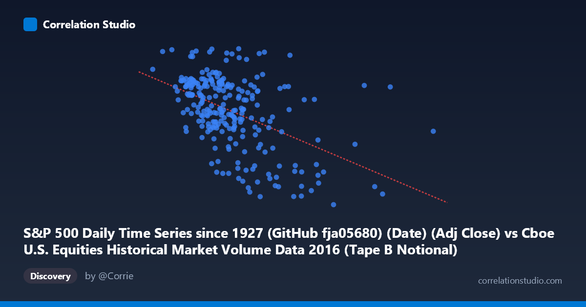
S&P 500 Daily Time Series since 1927 (GitHub fja05680) (Date) (Adj Close) vs Cboe U.S. Equities Historical Market Volume Data 2016 (Tape B Notional)

Pearson correlation (r): -0.4865
Spearman correlation: -0.4684
p-value: 0
Sample size (n): 252
95% confidence interval: -0.5755 to -0.3861
Granger causality: None
Granger optimal lag: 1

AI analysis

Analysis: S&P 500 Adjusted Close vs. Cboe Tape B Notional Volume (2016)

Relationship Overview The scatterplot reveals a moderate negative relationship between S&P 500 adjusted closing prices and Cboe Tape B notional trading volume throughout 2016. As S&P 500 prices increased, Tape B notional volume tended to decrease, and conversely, periods of lower index prices were associated with higher notional volumes. This pattern is consistent with a well-documented market microstructure phenomenon: elevated volatility and fear-driven selling during price declines generate disproportionately high notional trading activity, while steadily rising markets often see more subdued, complacent volume profiles.

Correlation Strength and Statistical Significance The Pearson correlation of r = -0.49 indicates a moderate negative association, with the linear regression (y = -3.16×10⁻⁸x + 2254.22) confirming the downward slope. However, r² = 0.237 means that S&P 500 price levels explain only about 23.7% of the variance in Tape B notional volume — leaving more than three-quarters of the variation attributable to other factors. The 95% confidence interval of [-0.58, -0.39] is entirely negative and relatively tight, providing strong directional confidence, and the p-value of 2.22×10⁻¹⁶ confirms this is not a chance finding at any conventional significance threshold. Despite this statistical robustness, the Granger causality results are notably absent in both directions (X→Y: F=0.52, p=0.47; Y→X: F=0.09, p=0.76), meaning neither variable meaningfully predicts the other's future values at a one-period lag. This is a critical distinction: while a contemporaneous correlation exists, there is no evidence of temporal predictive causality, limiting any trading signal interpretation.

Notable Patterns, Clusters, and Outliers Several structural features stand out in the data. The bulk of observations cluster in the X range of roughly 3.5–5.5 billion, with Y values concentrated between 2,050 and 2,200, forming a relatively dense core. However, a distinct cluster of high-X, low-Y outliers is visible — points like (8,200,813,716; 2,127), (8,084,440,928; 1,869), and (6,712,820,579; 1,883) represent sessions with exceptionally high notional volume coinciding with depressed S&P prices, likely corresponding to volatile market events in early 2016 (the January–February selloff) or post-Brexit turbulence. Conversely, the point (6,299,758,519; 2,262) is a notable exception — high volume and high price — potentially representing the post-election rally in November 2016. The relationship also appears to have a slight non-linear or heteroscedastic character: variance in Y appears wider at lower X values, suggesting the negative relationship may be driven more by extreme volume episodes than by a uniform linear mechanism.

Confounding Factors and Caveats Several important caveats apply. First, Tape B specifically covers NYSE American (AMEX)-listed securities, not the full market, so its notional volume dynamics may differ from aggregate market behavior and may not directly reflect S&P 500 constituent trading. Second, the negative correlation may be substantially driven by regime-specific episodes — market stress events that simultaneously depress prices and spike volumes — rather than a structural, persistent relationship. Removing the handful of extreme high-volume outliers would likely weaken the correlation considerably. Third, notional volume is price-sensitive by construction: if prices fall, the same number of shares traded produces lower notional value, which could introduce a mechanical negative bias into the correlation that overstates the behavioral signal. Finally, 2016 was an unusual year with identifiable macro shocks (oil price collapse, Brexit, U.S. election), making generalization to other periods risky.

Actionable Insights and Further Investigation Practitioners should not use S&P 500 price levels as a predictive input for next-day Tape B notional volume, given the failed Granger causality tests — the relationship is contemporaneous, not anticipatory. More productive next steps would include: (1) decomposing the analysis by market regime (low vs. high VIX environments) to test whether the correlation strengthens during stress periods; (2) replacing notional volume with share volume or trade count to isolate the mechanical price-notional artifact; (3) extending the time series beyond 2016 to test whether this relationship is stable or year-specific; and (4) incorporating implied volatility (VIX) as a mediating variable, which likely explains a substantial portion of both variables' variance simultaneously and may reduce or eliminate the apparent direct correlation between price and volume.

X dataset: Cboe U.S. Equities Historical Market Volume Data 2016

Y dataset: S&P 500 Daily Time Series since 1927 (GitHub fja05680) (Date)

Part of experiment: Daily - Cboe U.S. Equities Historical Market Volume Data 2016 vs S&P 500 Daily Time Series since 1927 (GitHub fja05680) (Date)