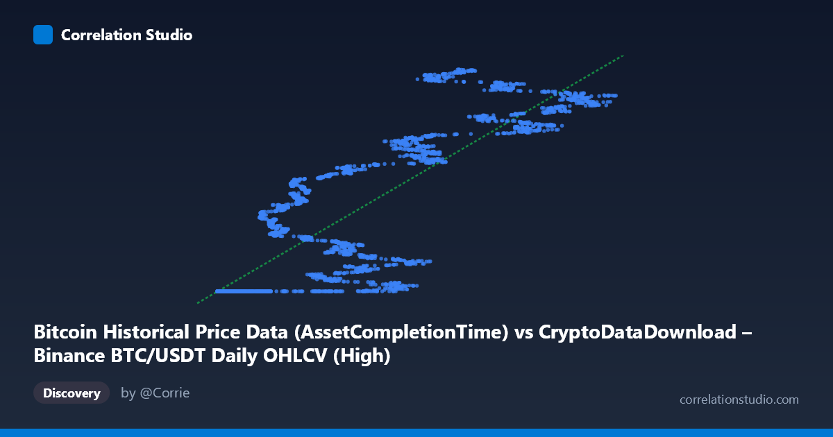
Bitcoin Historical Price Data (AssetCompletionTime) vs CryptoDataDownload – Binance BTC/USDT Daily OHLCV (High)
- Pearson correlation (r)
- 0.85
- Spearman correlation
- 0.886
- p-value
- 0
- Sample size (n)
- 3191
- 95% confidence interval
- 0.8401 to 0.8593
- Granger causality
- None
- Granger optimal lag
- 10
AI analysis
Analysis of Bitcoin Price/Time-Related Metric Correlation
1. Overview of the Relationship
The scatterplot reveals a strong positive, but distinctly non-linear relationship between the X variable (AssetCompletionTime, appears to represent an elapsed-time or processing-time metric) and Y (BTC/USDT daily High price). Rather than a diffuse cloud of points, the data shows a clear stepped or clustered structure: a large mass of points sits at low X values (roughly 3,000–25,000) with Y compressed tightly near the minimum (~1,614,337,000–1,614,338,000), followed by a rising staircase pattern as X increases toward 60,000–126,000, with Y climbing toward 1,780,000,000. This suggests the relationship is driven by regime shifts or discrete time periods rather than a smooth continuous association.
2. Strength, Direction, and Statistical Confidence
The Pearson correlation of r = 0.85 indicates a strong positive linear association, and r² = 0.7225 means approximately 72% of the variance in Y is explained by X in a simple linear model — leaving a substantial 28% unexplained, consistent with the visible non-linear clustering. The 95% confidence interval [0.8401, 0.8593] is narrow, reflecting the large sample size (n=3,191) and giving high confidence that the true population correlation is robustly positive; the p-value of 0 confirms this is not a chance result. However, the Granger causality tests show no significant predictive direction in either direction (X→Y: p=0.31; Y→X: p=0.13). This is a critical caveat: despite strong contemporaneous correlation, neither variable helps forecast the other's future values beyond its own history. This strongly suggests the correlation is not causal in a temporal-predictive sense but likely reflects a shared underlying trend (e.g., both variables increasing together over the 2017–2026 time span, possibly both indexed to date/time).
3. Notable Patterns and Outliers
The most striking feature is the flat-line cluster at low X (many points near Y≈1,614,337,000–1,614,338,000) — this looks like a floor/boundary effect or a repeated constant value, possibly representing an early period (e.g., BTC's 2017 lows) where many observations share nearly identical Y values despite varying X. Beyond this cluster, the data forms discrete rising bands (~1,660M, ~1,690M, ~1,710M, ~1,740M, ~1,775M), suggestive of price plateaus or step-function behavior rather than continuous covariation — possibly artifacts of how "High" prices cluster within trading ranges or resistance levels during different market phases. No extreme outliers are apparent; the pattern is more consistent with quantized/regime-based clustering than random scatter.
4. Confounding Factors and Caveats
Both variables appear time-dependent (X may itself be a timestamp-derived metric), meaning the apparent correlation is likely confounded by a common time trend — both series may simply be trending upward across the 2017–2026 window independent of any direct mechanistic link. This is a classic case of spurious correlation via co-trending non-stationary time series, especially relevant for financial/crypto data. The lack of Granger causality reinforces that this is not a genuine leading/lagging predictive relationship. Additionally, mixing two differently-sourced datasets (CDD OHLCV vs. a separate "Historical Price Data" column) risks alignment/merge artifacts, especially given the flat cluster suggesting duplicated or forward-filled values.
5. Recommendations for Further Investigation
To clarify whether this is genuine or spurious: (1) detrend or difference both series (e.g., use returns/percentage changes instead of levels) and recompute correlation — true price-driving relationships should persist after removing shared trends; (2) investigate the flat-line cluster to confirm whether it reflects legitimate 2017 data or a data-quality/fill-forward artifact; (3) consider piecewise or segmented regression to model the apparent regime shifts rather than a single linear fit; (4) verify X's actual definition (timestamp vs. duration) since "AssetCompletionTime" is ambiguous and critical for correct causal interpretation.
X dataset: CryptoDataDownload – Binance BTC/USDT Daily OHLCV
Y dataset: Bitcoin Historical Price Data
Part of experiment: Bitcoin - CryptoDataDownload – Binance BTC/USDT Daily OHLCV vs Bitcoin Historical Price Data