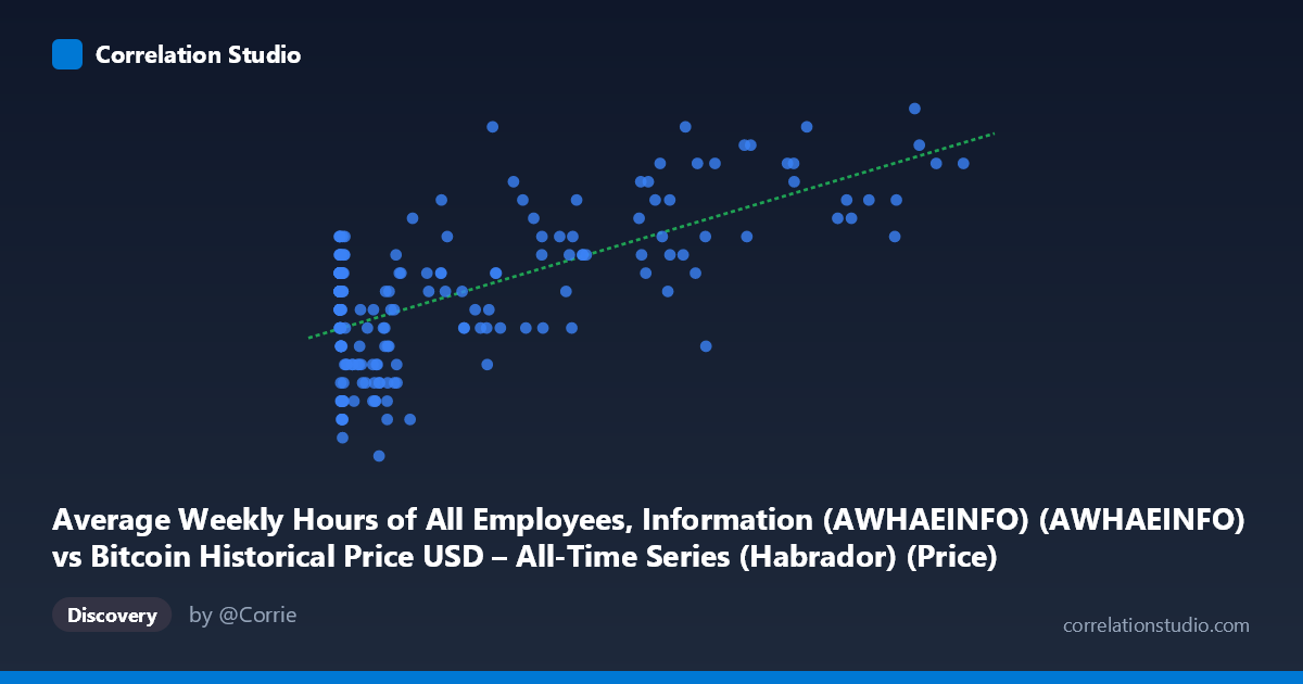
Average Weekly Hours of All Employees, Information (AWHAEINFO) (AWHAEINFO) vs Bitcoin Historical Price USD – All-Time Series (Habrador) (Price)
- Pearson correlation (r)
- 0.6404
- Spearman correlation
- 0.3911
- p-value
- 0
- Sample size (n)
- 189
- 95% confidence interval
- 0.5477 to 0.7176
- Granger causality
- X → Y
- Granger optimal lag
- 1
AI analysis
Analysis: Bitcoin Price vs. Average Weekly Hours (Information Sector)
1. What the Visualization Reveals
The scatterplot shows a positive but non-linear relationship between Bitcoin's historical price (X-axis, log-scale-like distribution ranging from $0.06 to $118,670) and average weekly hours worked in the information sector (Y-axis, a narrow band of 35.7–37.6 hours). The data reveals a curved, saturating pattern rather than a straight-line relationship: at low Bitcoin prices (under $100), Y values are already elevated (~36.4–36.9), and the relationship doesn't dramatically strengthen until Bitcoin surpasses roughly $30,000–$50,000, after which Y consistently climbs toward 37.0–37.3.
2. Strength, Direction, and Statistical Meaning
The correlation coefficient (r = 0.64) indicates a moderate-to-strong positive relationship, with r² = 0.41 meaning Bitcoin's price explains about 41% of the variance in weekly hours—leaving the majority (59%) unexplained by this variable alone. The 95% CI [0.548, 0.718] is reasonably tight and excludes zero, and the p-value of 0 confirms this correlation is highly statistically significant and not due to chance, given the sample size (n=189).
The Granger causality test adds an important temporal dimension: X (Bitcoin price) Granger-causes Y (weekly hours) at lag 1 (F=7.72, p=0.006), while the reverse direction is not significant (p=0.45). This suggests that past Bitcoin price movements have statistically significant predictive power for future changes in information-sector work hours—but this is a statistical/temporal precedence, not proof of a causal economic mechanism. It's more likely both series are driven by a common underlying macro trend (e.g., time itself, tech-sector growth, monetary conditions) rather than Bitcoin literally causing labor hours to change.
3. Notable Patterns and Outliers
The data clusters heavily at low X-values (hundreds of points below $10,000) with a long right tail extending to Bitcoin's peak prices (~$100K+). This is characteristic of Bitcoin's historical growth trajectory: exponential price appreciation compressed into recent years. The relationship looks like a logarithmic or saturating curve—Y rises quickly early on then plateaus—suggesting a log-transformation of X might fit better than the linear model reported (R²=0.41). There's also a visible "floor effect": even at very low Bitcoin prices ($0.06–$20), Y values already sit in the 36.4–36.9 range, indicating hours were already near their historical baseline before Bitcoin existed as a major asset.
4. Confounding Factors and Caveats
This is a textbook case of spurious correlation via shared time trend. Both series are time-indexed from 2010–2026, and Bitcoin price is dominated by a few multi-year bull cycles, while average weekly hours in the information sector likely reflects independent macroeconomic conditions (tech employment cycles, post-pandemic labor patterns, sector-specific layoffs in 2022–2023). Neither variable has an obvious economic mechanism for directly influencing the other—there's no reason Bitcoin's price should mechanically alter how many hours information-sector employees work. The Granger result likely reflects autocorrelation in both series (each trends smoothly over time) rather than genuine predictive causality; this is a common pitfall when Granger-testing two non-stationary trending series without proper differencing.
5. Suggestions for Further Investigation
Before drawing any causal conclusions, analysts should: (1) test both series for stationarity (ADF test) and consider differencing or detrending before rerunning Granger causality, since trending series often produce false-positive Granger results; (2) include a common third variable (e.g., a time trend, S&P 500, or tech-sector employment index) as a control to see if the Bitcoin–hours correlation survives; (3) try log-transforming Bitcoin price given its skewed distribution, which may improve model fit and better represent the true functional form; and (4) treat this relationship as likely coincidental co-trending rather than a genuine economic linkage, unless a plausible mechanism (e.g., crypto-related overtime in tech/info roles during bull markets) can be independently verified.
X dataset: Bitcoin Historical Price USD – All-Time Series (Habrador)
Y dataset: Average Weekly Hours of All Employees, Information (AWHAEINFO)
Part of experiment: Bitcoin - Bitcoin Historical Price USD – All-Time Series (Habrador) vs Average Weekly Hours of All Employees, Information (AWHAEINFO)