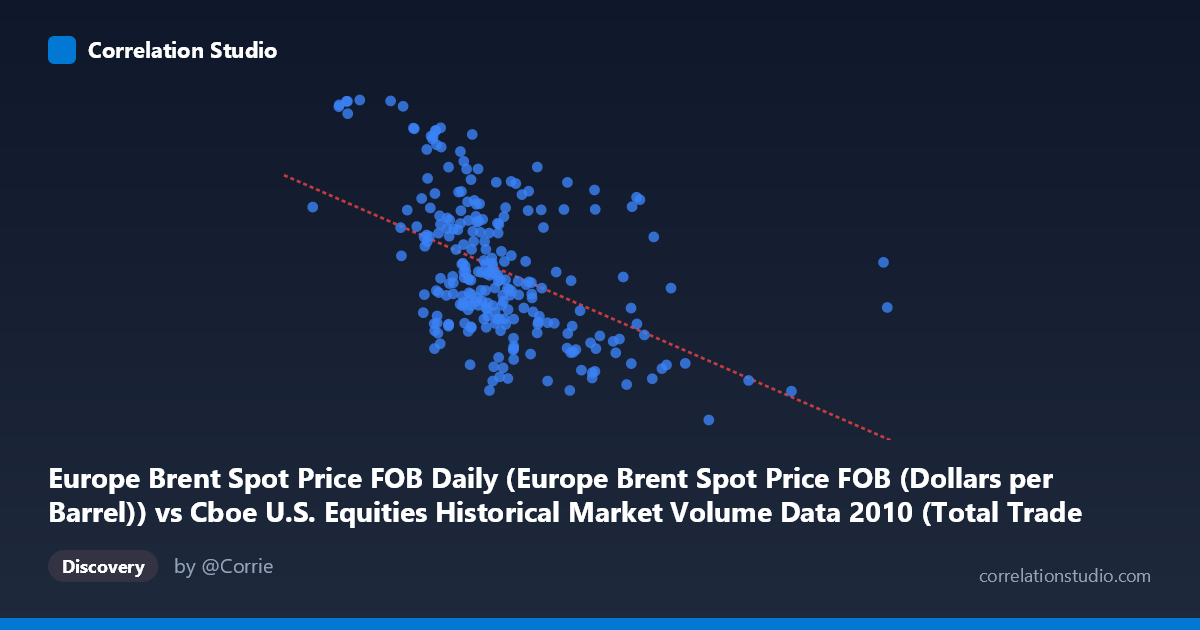
Europe Brent Spot Price FOB Daily (Europe Brent Spot Price FOB (Dollars per Barrel)) vs Cboe U.S. Equities Historical Market Volume Data 2010 (Total Trade Count)
- Pearson correlation (r)
- -0.484
- Spearman correlation
- -0.4855
- p-value
- 0
- Sample size (n)
- 252
- 95% confidence interval
- -0.5733 to -0.3834
- Granger causality
- None
- Granger optimal lag
- 1
AI analysis
Analysis: Europe Brent Spot Price vs. U.S. Equities Total Trade Count (2010)
Relationship Overview
The scatterplot reveals a negative relationship between Europe Brent crude oil spot prices (X-axis, in dollars per barrel) and U.S. equities total trade count (Y-axis), meaning that as oil prices rose during 2010, the number of equity trades tended to decline. The linear regression equation (y = -4.27×10⁻⁶x + 89.15) confirms this downward slope, though the scatter around the regression line is substantial. This pattern is counterintuitive at first glance — one might expect higher oil prices to drive more market activity — but likely reflects broader macroeconomic dynamics of 2010, where rising commodity prices coincided with periods of relative market calm following the post-crisis volatility spike of 2008–2009.
Correlation Strength and Statistical Significance
The Pearson correlation of r = -0.484 indicates a moderate negative association, but the explanatory power is modest: r² = 0.234, meaning only about 23.4% of the variance in trade counts is explained by oil price levels. While statistically robust — the p-value of 2.22×10⁻¹⁶ is essentially zero across a sample of 252 paired observations drawn from a population of 3,302 — the 95% confidence interval of [-0.573, -0.383] confirms the effect is consistently negative but meaningfully uncertain in magnitude. Practically, this means roughly three-quarters of the variation in equity trade counts is driven by factors entirely unrelated to oil prices. The Granger causality tests add a critical caveat: neither direction achieves conventional significance at the 5% level (X→Y: F=0.58, p=0.447; Y→X: F=3.62, p=0.058), meaning oil prices do not temporally predict trade counts, nor vice versa, with any statistical confidence. The correlation is contemporaneous rather than predictive.
Notable Patterns, Clusters, and Outliers
Several features stand out in the sample data. There is a notable cluster of observations concentrated in the X range of roughly 1.5M–2.5M (notional volume units) with trade counts spanning 72–92, suggesting this represents the most common market regime during 2010. A handful of high-leverage outliers are visible: the point at approximately (1,046,906, 93.63) and (1,308,179, 93.55) represent unusually high trade counts at relatively low oil-price-correlated volumes, pulling the regression line and potentially inflating the correlation magnitude. Conversely, (4,002,972, 67.18) and (4,340,243, 70.45) anchor the lower-right of the distribution with high X and low Y values, reinforcing the negative slope. There is also a suggestion of non-linearity — the relationship appears steeper at lower X values and flattens at higher values — which a simple linear fit may not adequately capture.
Confounding Factors and Caveats
Several important caveats limit causal interpretation. 2010 was a structurally unusual year for U.S. equity markets — characterized by the Flash Crash (May 6, 2010) and residual post-financial-crisis behavioral shifts — meaning high trade counts at certain periods likely reflect fear/volatility rather than normal market function. Both variables are also driven by common macro factors: risk appetite, Federal Reserve policy, and global economic recovery momentum simultaneously affected oil demand and equity market participation, making it difficult to disentangle their relationship from shared confounders. Additionally, the axis labeling appears swapped between datasets in the metadata (X-axis pulls from the equities dataset while Y-axis pulls from the oil price dataset), which warrants verification before drawing firm conclusions. The lack of Granger causality also strongly suggests this correlation is spurious or coincidental at the temporal resolution tested.
Actionable Insights and Further Investigation
Given the moderate but unexplained variance, several investigative paths are warranted. First, introduce VIX (volatility index) as a control variable — it is likely a primary confounder driving both trade count surges and oil price reactions simultaneously. Second, test non-linear models (e.g., polynomial or piecewise regression) to determine whether the relationship changes character across different oil price regimes. Third, isolate the Flash Crash period (around May 2010) and re-run the analysis to assess whether the correlation is largely an artifact of that single high-volatility event. Fourth, extending the Granger causality test to longer lags (5–10 periods) may reveal delayed transmission effects not visible at lag 1. Finally, disaggregating trade counts by exchange type or sector (energy stocks vs. broader market) could reveal whether the correlation is concentrated in energy-related equities, which would provide a far more economically coherent narrative.
X dataset: Cboe U.S. Equities Historical Market Volume Data 2010
Y dataset: Europe Brent Spot Price FOB Daily
Part of experiment: Daily - Cboe U.S. Equities Historical Market Volume Data 2010 vs Europe Brent Spot Price FOB Daily