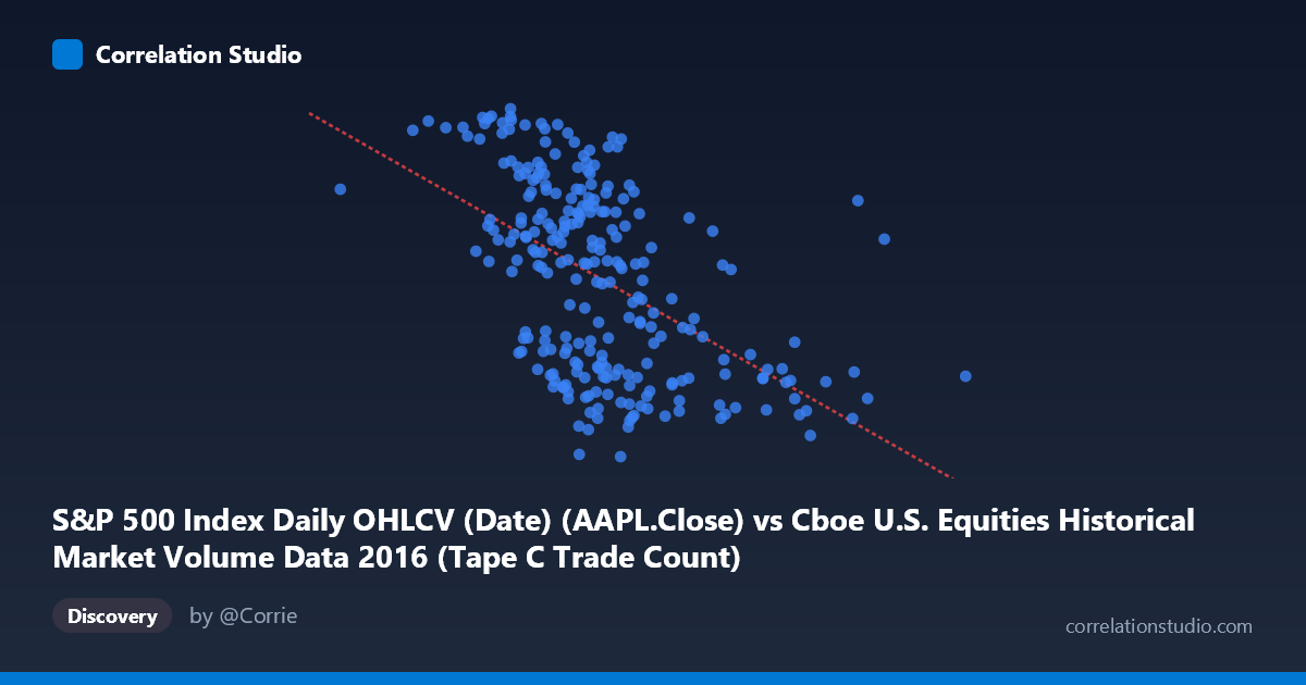
S&P 500 Index Daily OHLCV (Date) (AAPL.Close) vs Cboe U.S. Equities Historical Market Volume Data 2016 (Tape C Trade Count)

Pearson correlation (r): -0.5217
Spearman correlation: -0.5548
p-value: 0
Sample size (n): 252
95% confidence interval: -0.6062 to -0.4256
Granger causality: None
Granger optimal lag: 1

AI analysis

Analysis: AAPL Close Price vs. Cboe Tape C Trade Count (2016)

1. What the Visualization Reveals

The scatterplot displays a negative relationship between Apple's daily closing price (X-axis) and the Cboe U.S. Equities Tape C trade count (Y-axis) across 252 trading days in 2016. As AAPL's closing price increases, the number of trades on Tape C tends to decrease. The linear regression equation (y = -2.726×10⁻⁵x + 124.051) confirms this inverse slope, suggesting that for every $10 increase in AAPL's price, Tape C trade count declines by roughly 0.27 units on the index scale used. The data cloud spans a fairly wide range, with AAPL prices running from roughly $278K to $1.32M in the scaled units shown, and trade counts ranging from approximately 90 to 118 — indicating meaningful variability in both dimensions throughout the year.

2. Correlation Strength, Direction, and Temporal Causality

The Pearson correlation of r = -0.5217 indicates a moderate negative association, and the r² of 0.2722 tells us that only about 27.2% of the variance in Tape C trade counts is explained by AAPL's closing price — meaning roughly 72.8% of the variation remains unexplained by this linear relationship alone. While statistically robust (p ≈ 0, 95% CI: [-0.6062, -0.4256]), the confidence interval confirms the effect is reliably negative but stops well short of a strong correlation. Critically, the Granger causality results are non-significant in both directions (X→Y: F = 0.983, p = 0.322; Y→X: F = 0.690, p = 0.407), meaning neither variable meaningfully predicts the other's future values with a one-period lag. This strongly cautions against any causal or predictive interpretation — the contemporaneous correlation exists, but there is no detectable temporal lead-lag structure between these series.

3. Notable Patterns, Clusters, and Outliers

Several features stand out in the sample data. The bulk of observations cluster in the AAPL price range of roughly $580K–$800K, where trade counts span the full Y-range (90–118), suggesting high dispersion at mid-range prices rather than a tight linear band. A handful of higher-price observations (e.g., ~$990K–$1.03M, ~$914K, ~$1.32M) consistently appear with lower trade counts (93–96 range), anchoring the negative slope at the upper end. Conversely, several lower-price points (e.g., $519K at 117.06, $563K at 114.06) show elevated trade counts, reinforcing the pattern. The wide vertical spread throughout the middle of the X-range indicates the relationship is noisy and heteroscedastic, with considerable unexplained variance especially in the $580K–$750K zone.

4. Confounding Factors and Interpretive Caveats

Several important caveats apply. First, market-wide effects in 2016 — including the U.S. presidential election, Federal Reserve rate decisions, and sector rotations — likely drove both AAPL prices and overall trading volumes simultaneously, making the observed correlation potentially spurious or confounded by common macro drivers. Second, the axis labeling appears inverted in the dataset metadata (AAPL.Close is attributed to the Cboe dataset and vice versa), which may reflect a data join artifact and warrants careful verification. Third, Tape C specifically covers NYSE Arca-listed securities, so its trade count reflects broader market activity beyond AAPL alone — the correlation may be capturing a general market condition (e.g., high AAPL prices coinciding with low-volatility, low-volume regimes) rather than any direct relationship. Finally, with r² at only 27%, omitted variables such as VIX levels, overall S&P 500 volume, or day-of-week effects are likely substantial drivers.

5. Actionable Insights and Further Investigation

Given the moderate correlation without Granger causality, this relationship should not be used for predictive modeling in its current form. Recommended next steps include: (1) controlling for macro variables (VIX, S&P 500 daily volume, market regime) using multiple regression to determine whether the AAPL-Tape C relationship survives adjustment; (2) testing longer Granger lags (2–5 periods) to rule out delayed predictive relationships; (3) segmenting the data by market regime or quarter, as the 2016 election period may have created a structural break distorting the annual correlation; and (4) verifying the dataset column assignment to rule out any metadata mismatch. Exploring non-linear models (e.g., polynomial or spline regression) may also capture the apparent heteroscedasticity in the middle price range more effectively than the current linear specification.

X dataset: Cboe U.S. Equities Historical Market Volume Data 2016

Y dataset: S&P 500 Index Daily OHLCV (Date)

Part of experiment: Daily - Cboe U.S. Equities Historical Market Volume Data 2016 vs S&P 500 Index Daily OHLCV (Date)