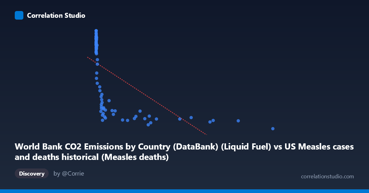
World Bank CO2 Emissions by Country (DataBank) (Liquid Fuel) vs US Measles cases and deaths historical (Measles deaths)
- Pearson correlation (r)
- -0.607
- Spearman correlation
- -0.8699
- p-value
- 0
- Sample size (n)
- 92
- 95% confidence interval
- -0.7221 to -0.4593
- Granger causality
- None
- Granger optimal lag
- 10
- Time coverage
- 1919-01-01 to 2020-01-01
- Recomputed on refreshed data
- 2026-10-17 (r was -0.607)
AI analysis
Scatterplot Analysis: CO2 Liquid Fuel Emissions vs. US Measles Deaths
1. Visual Relationship Overview
The scatterplot reveals a negative association between World Bank CO2 liquid fuel emissions and US measles deaths, with a clear hyperbolic or logarithmic decay pattern rather than a simple linear one. Data points cluster heavily at low X values (near zero) with high Y values (measles deaths in the thousands), while points at higher X values (higher emissions) tend to have substantially lower measles death counts. This visual shape — a steep initial drop that flattens asymptotically — is a hallmark of a logarithmic or power-law relationship rather than a linear one, which is consistent with the note that Spearman's ρ exceeds Pearson's r. The linear regression line (y = -1.099x + 9611.94) captures the general trend but visibly underfits the curvature in the data.
2. Correlation Strength, Direction, and Predictive Value
The Pearson correlation of r = -0.607 indicates a moderate-to-strong negative correlation, but the R² of 0.3685 means that only about 36.8% of the variance in measles deaths is statistically explained by CO2 liquid fuel emissions. The remaining ~63% is attributable to other factors entirely. The 95% confidence interval of [-0.722, -0.459] is meaningfully narrow and does not cross zero, confirming the association is robust, and the p-value of 1.41 × 10⁻¹⁰ is highly statistically significant — this correlation is extremely unlikely to be a chance artifact given the sample size of 92 paired observations. However, the Granger causality results are unambiguous in their non-significance: neither direction (X→Y nor Y→X) shows predictive power (F = 0.82, p = 0.61 and F = 0.38, p = 0.95, respectively, at an optimal lag of 10 periods). This means that despite the strong contemporaneous correlation, neither variable temporally predicts the other, which is a critical caveat against any causal interpretation.
3. Notable Patterns, Clusters, and Outliers
Several structural features stand out:
- Left-side cluster: The majority of points pile up at X ≈ 0–500, with measles deaths ranging from ~1,900 to ~13,600. This dense cluster dominates the regression and likely drives much of the correlation signal. - High-emission outliers: Points at extreme X values (e.g., X = 12,992 with Y = 1,457; X = 10,450 with Y = 2,432; X = 8,607 with Y = 2,475) are consistent with the trend but represent an era of near-zero measles mortality — these are likely post-vaccine era years (post-1963). - High-death anomalies: Several points with very low X but moderate Y (e.g., (24, 7,691), (41, 8,348), (81, 7,079), (261, 6,636)) fall noticeably below the main high-death cluster, suggesting within-era variation in measles mortality that emissions alone cannot explain. - The non-linear shape: The data strongly suggest a logarithmic fit would be more appropriate (log(X+1) as a predictor), which would likely improve R² substantially and reduce heteroscedasticity in the residuals.
4. Confounding Factors and Interpretive Caveats
This correlation is almost certainly a spurious time-series coincidence driven by a shared temporal trend rather than any mechanistic link. Both variables are proxies for historical era:
- Measles deaths declined dramatically due to improved healthcare (1930s–1950s), the introduction of the measles vaccine in 1963, and better public health infrastructure — all time-indexed phenomena. - CO2 liquid fuel emissions grew steadily through the 20th century due to industrialization, automobile adoption, and economic expansion — also strongly time-indexed. - The confounding variable is time itself (or the broader construct of 20th-century modernization). Any variable that increased monotonically from 1919 to 2020 would correlate negatively with measles deaths. - The Granger causality null result reinforces this: there is no temporal lead-lag relationship, which would be expected if one variable genuinely influenced the other. - The mismatch between dataset labels (CO2 data listed under measles dataset and vice versa) warrants verification that the correct columns were joined.
5. Actionable Insights and Further Investigation
- Apply a logarithmic transformation to X (e.g., log(CO2 + 1)) before re-fitting; this would better capture the hyperbolic decay visible in the scatterplot and likely raise R² considerably. - Introduce time as an explicit variable or use a partial correlation controlling for year to test whether the r = -0.607 survives after removing the shared time trend — it almost certainly would collapse substantially. - Segment the analysis into pre-vaccine (pre-1963) and post-vaccine eras to determine whether any within-era association exists, which would be more meaningful than the pooled analysis. - Compare against mechanistically plausible variables (vaccination rates, healthcare spending, population density) to build a proper multivariate model for measles mortality. - This dataset pairing serves as an excellent pedagogical example of spurious correlation in time-series data — it may be worth documenting explicitly as a cautionary case study for analysts working with historical annual data.
X dataset: US Measles cases and deaths historical
Y dataset: World Bank CO2 Emissions by Country (DataBank)
Part of experiment: Yearly - US Measles cases and deaths historical vs World Bank CO2 Emissions by Country (DataBank)