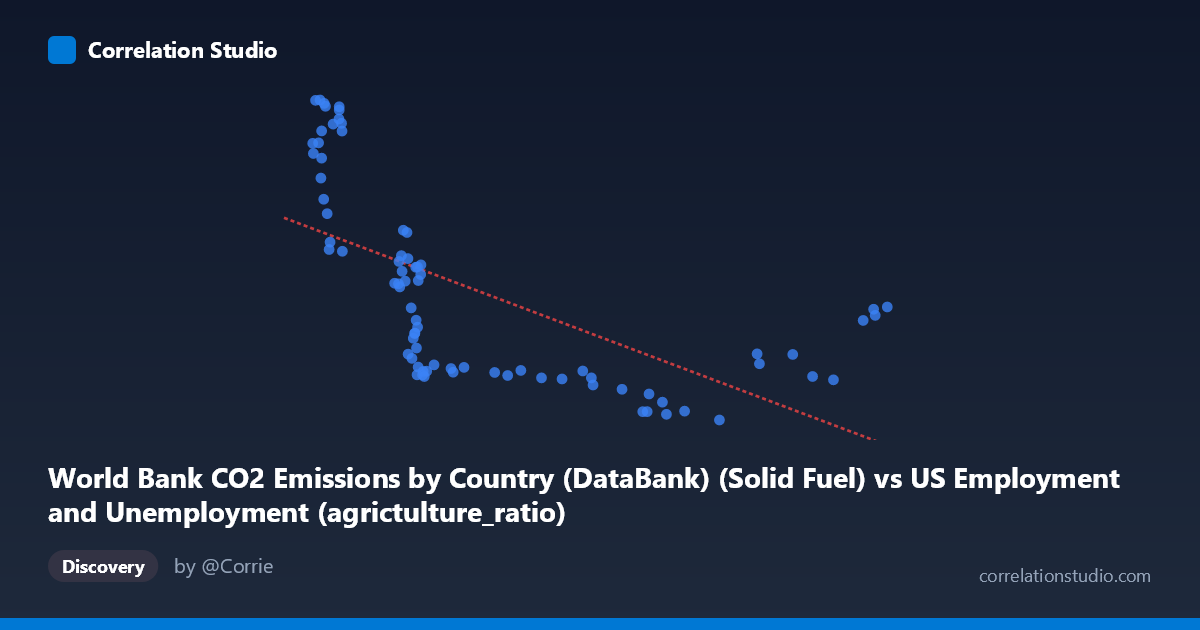
World Bank CO2 Emissions by Country (DataBank) (Solid Fuel) vs US Employment and Unemployment (agrictulture_ratio)
- Pearson correlation (r)
- -0.6245
- Spearman correlation
- -0.8316
- p-value
- 0
- Sample size (n)
- 80
- 95% confidence interval
- -0.7424 to -0.4692
- Granger causality
- None
- Granger optimal lag
- 10
- Time coverage
- 1941-01-01 to 2020-01-01
AI analysis
Scatterplot Analysis: Solid Fuel CO2 Emissions vs. US Agriculture Employment Ratio
1. Overall Relationship Revealed
The scatterplot reveals a negative relationship between World Bank solid fuel CO2 emissions and the US agriculture employment ratio, spanning data from 1941 to 2020. As solid fuel emissions increase, the proportion of the US workforce employed in agriculture tends to decrease. This broadly reflects a shared historical narrative: post-WWII industrialization drove both rising fossil fuel consumption and the mechanization of agriculture, which systematically reduced the need for agricultural labor. The linear regression equation (y = −2.04x + 26,753.5) captures this downward slope, though the scatter around the line is considerable, hinting that the relationship is not cleanly linear.
2. Correlation Strength, Direction, and Statistical Framing
The Pearson correlation of r = −0.6245 indicates a moderate-to-strong negative association, but the R² of 0.39 means only 39% of the variance in the agriculture employment ratio is explained by solid fuel emissions — leaving 61% attributable to other forces. The 95% confidence interval of [−0.74, −0.47] is entirely negative, confirming the direction is reliable, and the p-value of 5.999×10⁻¹⁰ makes this result highly statistically significant, effectively ruling out chance. However, statistical significance does not imply practical or causal significance. Critically, Granger causality tests find no significant predictive direction in either direction (X→Y: p = 0.63; Y→X: p = 0.10), meaning neither variable temporally predicts the other after accounting for lags up to 10 periods. This strongly cautions against any causal interpretation.
3. Notable Patterns, Clusters, and Non-Linear Features
The scatterplot displays several visually distinct features. A dense cluster of points appears at lower X values (roughly 2,095–3,500) with high and widely spread Y values (agriculture ratios of ~12,000–31,000), suggesting high variability in early decades when agricultural employment was still transitioning. A second cluster emerges at higher X values (6,000–9,250) where Y values compress into a narrower band (~9,500–17,000), indicating that once emissions scaled up in later decades, agriculture ratios had already stabilized at lower levels. Several high-leverage outliers are visible at low X with very high Y (e.g., ~2,186; 31,154 and ~2,130; 31,132), likely representing early 1940s observations. Importantly, the Spearman ρ exceeding Pearson r explicitly flags a non-linear relationship — a logarithmic or power curve would likely fit this data better than the linear model, particularly given the rapid early decline that appears to flatten at higher emission levels.
4. Confounding Factors and Interpretive Caveats
This correlation is almost certainly driven by mutual dependence on time rather than any direct causal mechanism between solid fuel emissions and agricultural employment. Both variables are time-indexed from 1941–2020, making common temporal trends (technological change, urbanization, post-war economic growth, energy infrastructure expansion) the dominant confounding factor. The dataset labeling also raises concerns: the X-axis column ("Solid Fuel CO2 Emissions") comes from a US employment dataset, while the Y-axis ("agricultureratio") comes from the World Bank CO2 dataset — suggesting these may have been joined across different source datasets, introducing potential alignment or unit inconsistencies. Additionally, the agriculture ratio metric is not defined in standard units here, and its scale (~9,500–31,000) is atypical for a simple employment percentage, warranting scrutiny. The absence of Granger causality at lags up to 10 years further reinforces that this is a spurious correlation mediated by shared historical trends.
5. Actionable Insights and Further Investigation
Given the likely spurious nature of this correlation, the priority should be detrending both time series (e.g., first-differencing or removing a common time trend) before drawing any substantive conclusions. A logarithmic regression should be tested given the Spearman/Pearson discrepancy, as the relationship appears to saturate at higher emission levels. Further investigation should introduce explicit time as a covariate or use structural break analysis to identify whether the relationship changes across distinct economic eras (e.g., pre/post-1970s energy crisis). Researchers should also verify the unit definitions and dataset join logic to ensure the agriculture ratio and emissions figures are temporally and geographically aligned. Finally, comparing this pattern against other countries' agricultural employment trends could help distinguish whether this reflects a US-specific structural shift or a broader global industrialization signature.
X dataset: US Employment and Unemployment
Y dataset: World Bank CO2 Emissions by Country (DataBank)
Part of experiment: Yearly - US Employment and Unemployment vs World Bank CO2 Emissions by Country (DataBank)