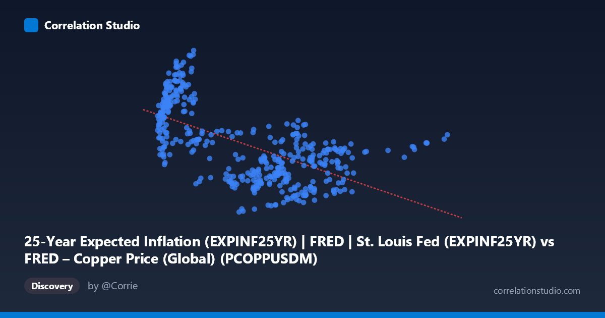
25-Year Expected Inflation (EXPINF25YR) | FRED | St. Louis Fed (EXPINF25YR) vs FRED – Copper Price (Global) (PCOPPUSDM)
- Pearson correlation (r)
- -0.6162
- Spearman correlation
- -0.5932
- p-value
- 0
- Sample size (n)
- 417
- 95% confidence interval
- -0.6724 to -0.5529
- Granger causality
- None
- Granger optimal lag
- 1
- Time coverage
- 1992-01-01 to 2026-09-01
- Recomputed on refreshed data
- 2026-10-27 (r was -0.6328)
AI analysis
Analysis: Copper Price vs. 25-Year Expected Inflation
1. Overview of the Relationship
The scatterplot shows a moderate-to-strong negative relationship between copper prices (X-axis, ranging from ~$1,377 to ~$12,987/metric ton) and 25-year expected inflation (Y-axis, ranging from 1.67% to 3.63%). As copper prices rise, long-term inflation expectations tend to decline — a counterintuitive pattern given copper's traditional role as an inflation-sensitive industrial commodity ("Dr. Copper"). The data points at low copper prices (under $3,000) cluster tightly around higher inflation expectations (2.8%–3.5%), while higher copper prices (above $7,000) correspond to a wider but lower band of expectations (1.8%–2.5%).
2. Strength, Direction, and Statistical Confidence
The correlation coefficient (r = -0.657) indicates a moderate-to-strong negative linear relationship, with r² = 0.432, meaning copper price explains about 43% of the variance in 25-year inflation expectations — leaving the majority (57%) unexplained by this simple linear relationship. The 95% CI [-0.709, -0.598] is fairly tight and does not cross zero, and the p-value (~0) confirms this relationship is highly statistically significant and not due to chance, given the large sample (n=411). However, the Granger causality results are critical: neither variable significantly predicts the other in a temporal/lagged sense (X→Y: p=0.895; Y→X: p=0.991). This strongly suggests the correlation is not causal in a predictive sense — it likely reflects a shared response to a common underlying driver (e.g., macroeconomic regime, monetary policy cycles) rather than one variable leading the other.
3. Notable Patterns and Features
The relationship appears non-linear/regime-based rather than purely linear. Low copper prices (~$1,400–3,000) correspond almost exclusively to a distinct high-inflation-expectation cluster (2.8%–3.5%), likely reflecting an early-cycle period (possibly early 2000s or 2020-21 inflation scare with low copper). Mid-range copper prices ($4,000–6,000) show more variance (2.0%–2.6%). High copper prices ($7,000–10,000+) show a compressed, lower band (1.8%–2.5%) with less spread — suggesting a flattening or saturation effect at higher price levels rather than continued linear decline. This clustering pattern (visible in the sample data) hints at distinct time regimes/eras rather than a smooth continuous relationship, which the linear R² likely overstates in terms of a "true" mechanistic link.
4. Confounding Factors and Caveats
This is very likely a spurious or confounded time-series correlation rather than a direct causal link. Both series are probably driven by common macro factors: Federal Reserve monetary policy, global growth cycles, USD strength, and supply-chain dynamics. The 34-year time span (1992–2026) covers multiple distinct macroeconomic regimes (dot-com era, 2008 financial crisis, 2020-21 pandemic/inflation surge, tightening cycles) — pooling these into one correlation risks Simpson's paradox, where within-regime relationships could differ from or even contradict the pooled trend. Additionally, both variables are non-stationary trending time series; correlating levels (rather than changes/differences) inflates apparent correlation without implying genuine covariation.
5. Suggested Further Investigation
- Test for cointegration and re-run analysis on first-differences or year-over-year changes rather than levels, to control for shared trends/non-stationarity. - Segment by macro regime (e.g., pre/post-2008, pre/post-2020) to check whether the negative relationship holds within each era or is an artifact of pooling. - Investigate lagged relationships beyond 1 period — Granger tests at lag 1 show no causality, but longer lags (6-24 months) might reveal delayed pass-through effects given inflation expectations are forward-looking. - Introduce a third variable (real interest rates, USD index, Fed funds rate) as a likely common driver to test whether it explains the shared variance, converting this bivariate analysis into a more robust multivariate model.
X dataset: FRED – Copper Price (Global)
Y dataset: 25-Year Expected Inflation (EXPINF25YR) | FRED | St. Louis Fed
Part of experiment: Copper - FRED – Copper Price (Global) vs 25-Year Expected Inflation (EXPINF25YR) | FRED | St. Louis Fed