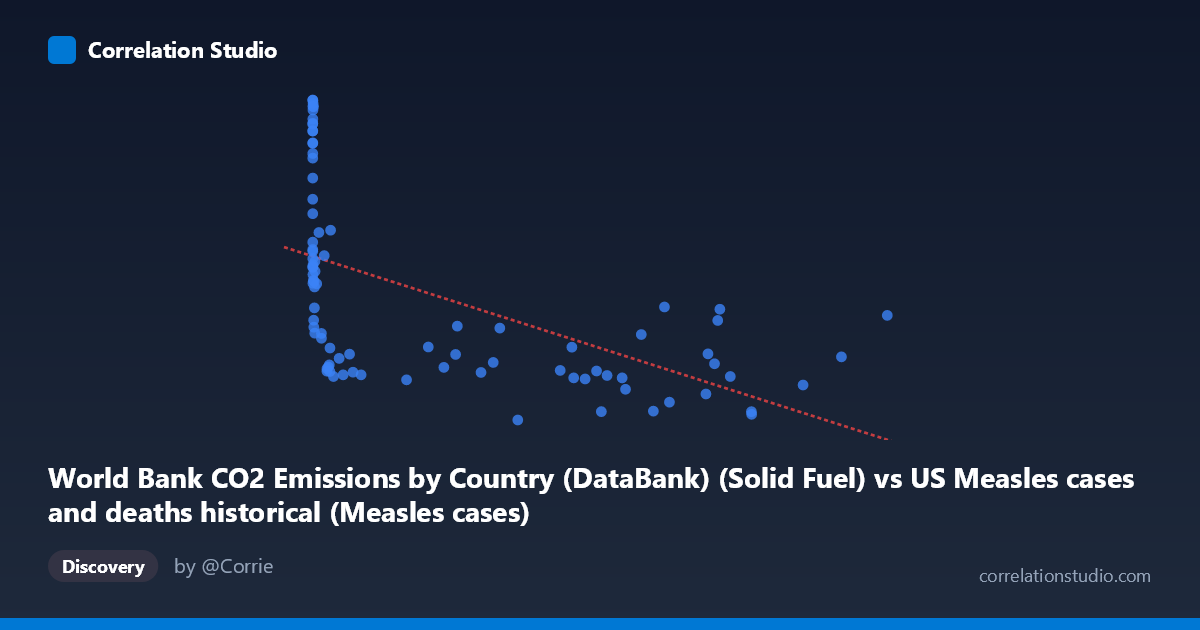
World Bank CO2 Emissions by Country (DataBank) (Solid Fuel) vs US Measles cases and deaths historical (Measles cases)
- Pearson correlation (r)
- -0.5578
- Spearman correlation
- -0.7991
- p-value
- 0
- Sample size (n)
- 87
- 95% confidence interval
- -0.6877 to -0.3934
- Granger causality
- None
- Granger optimal lag
- 10
AI analysis
Analysis of US Measles Cases vs. Solid Fuel CO2 Emissions
1. What the Visualization Reveals
The scatterplot displays a negative relationship between solid fuel CO2 emissions (X-axis) and US measles cases (Y-axis) spanning 1919–2020. The most visually striking feature is a pronounced bifurcation in the data: a dense cluster of high-Y values (measles cases roughly 19,000–31,000+) concentrated at very low X values (emissions below ~5,000 units), and a separate horizontal band of low-to-moderate Y values spread across the full range of X. This L-shaped or hyperbolic dispersion immediately signals that a simple linear model is an incomplete descriptor of the relationship, consistent with the note that Spearman ρ exceeds Pearson r.
2. Correlation Strength, Direction, and Causality
The Pearson r of −0.558 indicates a moderate negative correlation, but the R² of 0.311 means only 31.1% of the variance in measles cases is explained by solid fuel emissions—leaving nearly 69% attributable to other factors. The 95% confidence interval of [−0.688, −0.393] is entirely negative and does not cross zero, and the p-value of 1.99×10⁻⁸ confirms this is highly statistically significant; the correlation is almost certainly not a sampling artifact. However, statistical significance does not imply practical or causal significance here. Crucially, Granger causality testing finds no significant predictive direction in either direction (X→Y: F=0.798, p=0.631; Y→X: F=0.670, p=0.747 at optimal lag 10), meaning neither variable temporally predicts the other in any mechanistically meaningful way. This is a strong caution against causal interpretation.
3. Notable Patterns, Clusters, and Outliers
Several structural features deserve attention: - High-leverage low-X cluster: Points with X < ~5,000 span nearly the entire Y range (≈9,500–31,000), suggesting that in early decades when emissions were low, measles cases were highly variable and frequently extreme. Points like (55, 31153), (187, 31131), (667, 30926), and (1274, 30698) represent enormous measles burdens at negligible emission levels. - High-X suppression: For X ~200,000, Y values are consistently compressed into a narrow band of roughly 9,500–17,000, creating the characteristic "arm" of the L-shape. - Potential outliers: (894134, 16616) sits at the far right with a moderately elevated Y, and (319124, 9555) represents the lowest measles case count in the dataset. These anchor the regression line substantially. - The linear regression (y = −0.01385x + 20,607) is visibly pulled by the high-X cluster and underestimates Y at low X values significantly.
4. Confounding Factors and Caveats
This correlation almost certainly reflects parallel secular trends rather than any direct relationship between solid fuel combustion and measles transmission. Both variables are strongly time-indexed: measles cases declined dramatically through the 20th century due to vaccine introduction (1963), improved public health infrastructure, herd immunity campaigns, and reporting changes, while solid fuel CO2 emissions rose monotonically with industrialization. Any two variables following opposite long-term trends over the same era will produce a spurious negative correlation. Additional confounders include: changes in disease surveillance and case-reporting methodology, population growth (affecting both emissions and case counts), geopolitical disruptions (WWII affecting both industrial output and public health), and the fact that the datasets originate from fundamentally different domains (global emissions vs. US disease burden). The dataset label cross-contamination noted in the axis descriptions (each dataset appears mislabeled on the opposing axis) also warrants verification of data integrity before drawing conclusions.
5. Actionable Insights and Further Investigation
Given the spurious nature of this correlation, the most productive next steps would be: - Detrend both time series (e.g., first-differencing or HP filter) before re-computing correlation to remove shared secular trends and test whether any residual association persists. - Fit a logarithmic or power-law model (supported by the Spearman Pearson finding) to better characterize the non-linear shape, particularly the rapid Y-decline at low X values. - Segment the analysis by era (pre-vaccine <1963, post-vaccine 1963–2020) to test whether the correlation structure differs meaningfully across regimes. - Introduce proper causal variables for measles (vaccination coverage rates, population density, international travel) to build a meaningful explanatory model rather than relying on an emissions proxy. - Re-examine data provenance and labeling—the axis notes suggest possible dataset join errors that should be resolved before any policy or research conclusions are drawn.
X dataset: US Measles cases and deaths historical
Y dataset: World Bank CO2 Emissions by Country (DataBank)
Part of experiment: Yearly - US Measles cases and deaths historical vs World Bank CO2 Emissions by Country (DataBank)