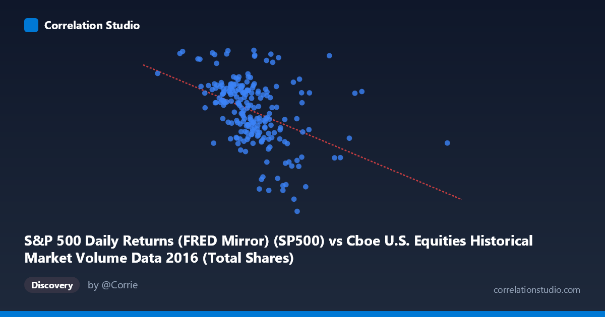
S&P 500 Daily Returns (FRED Mirror) (SP500) vs Cboe U.S. Equities Historical Market Volume Data 2016 (Total Shares)
- Pearson correlation (r)
- -0.4269
- Spearman correlation
- -0.4743
- p-value
- 0
- Sample size (n)
- 224
- 95% confidence interval
- -0.5284 to -0.3133
- Granger causality
- None
- Granger optimal lag
- 1
AI analysis
Scatterplot Analysis: S&P 500 Daily Returns vs. Cboe U.S. Equities Total Shares (2016)
Relationship Overview
The scatterplot reveals a moderate negative relationship between S&P 500 price levels (X-axis) and total shares traded on U.S. equities exchanges (Y-axis) across 2016. As the S&P 500 index value increases, total share volume tends to decrease — visually manifest as a downward-sloping point cloud. The linear regression equation (y = -3.469×10⁻⁷x + 2289.01) quantifies this: each one-unit increase in the S&P 500 index is associated with approximately a 0.000000347 decrease in total shares, which translates to meaningful volume reductions across the hundreds-of-millions range of observed index values. However, the scatter around this trend line is substantial, indicating that many individual observations deviate considerably from the predicted relationship.
Correlation Strength and Statistical Significance
The Pearson correlation of r = -0.4269 indicates a moderate negative association, but the explanatory power is limited: R² = 0.1822, meaning only about 18.2% of the variance in total share volume is explained by S&P 500 price level. The remaining ~82% is attributable to other factors entirely. The 95% confidence interval of [-0.5284, -0.3133] is reasonably narrow and does not include zero, reinforcing that the negative direction is reliable rather than a sampling artifact. The p-value of 2.461×10⁻¹¹ is extraordinarily small against a sample of n = 224 (drawn from N = 2,609), making it virtually certain this correlation did not arise by chance in the underlying population. That said, statistical significance should not be conflated with practical importance — a moderately correlated relationship explaining less than one-fifth of variance leaves the bulk of trading volume dynamics unexplained by price level alone.
Granger Causality and Temporal Directionality
Despite the statistically significant contemporaneous correlation, Granger causality tests find no significant predictive relationship in either direction at the optimal one-period lag. Neither X→Y (F = 0.2774, p = 0.5989) nor Y→X (F = 0.0015, p = 0.9692) reaches significance, strongly suggesting that past S&P 500 values do not help forecast future share volume, and vice versa. This is a critical finding: the correlation observed is likely driven by shared contemporaneous dynamics — both variables responding simultaneously to the same underlying market conditions — rather than one variable leading or driving the other. This distinction matters enormously for any predictive or causal interpretation of the relationship.
Notable Patterns, Clusters, and Outliers
Several features stand out in the sample data. The bulk of observations cluster in the X range of roughly 400M–550M with Y values between approximately 2050–2200 shares, forming a dense core. However, there are notable high-X outliers — points near 745M, 790M, and 807M on the X-axis — that correspond to relatively moderate Y values (roughly 2000–2163), consistent with the negative trend. Conversely, the point at X ≈ 200M (the minimum) yields Y ≈ 2213, among the higher share values — also consistent with the negative relationship. A few points appear to break the trend sharply: (656M, 1927) and (569M, 1948) sit well below the regression line, suggesting days of unusually low share volume despite moderate-to-high index values, potentially corresponding to specific market stress events or low-liquidity periods early in 2016. The spread of Y values at any given X is wide, reaffirming the low R².
Confounding Factors and Caveats
Several important caveats apply. First, the S&P 500 price level is not the same as daily returns — despite the dataset label referencing "Daily Returns," the X-axis values in the hundreds of millions suggest this column actually represents index price levels or notional values, not percentage returns. This potential mislabeling warrants verification before drawing conclusions. Second, time is a significant confound: both variables are time series spanning 2016, and the S&P 500 generally trended upward during this period while market structure changes (electronic trading evolution, regulatory shifts, volatility regimes) independently affected share volumes. The apparent negative correlation may partly reflect a spurious time-trend relationship rather than a true structural link. Third, known volatility events in early 2016 (market sell-off in January–February) likely produced high volume and lower prices simultaneously, driving the correlation, while calmer later periods saw higher prices and lower volume — making this relationship regime-dependent. For further investigation, analysts should: (1) control for the VIX or realized volatility to isolate the price-volume relationship from volatility effects; (2) test the relationship using S&P 500 returns (percent changes) rather than price levels to remove trend contamination; and (3) segment the data by market regime (high vs. low volatility periods) to assess whether the correlation is stable or driven primarily by specific episodes.
X dataset: Cboe U.S. Equities Historical Market Volume Data 2016
Y dataset: S&P 500 Daily Returns (FRED Mirror)
Part of experiment: Daily - Cboe U.S. Equities Historical Market Volume Data 2016 vs S&P 500 Daily Returns (FRED Mirror)