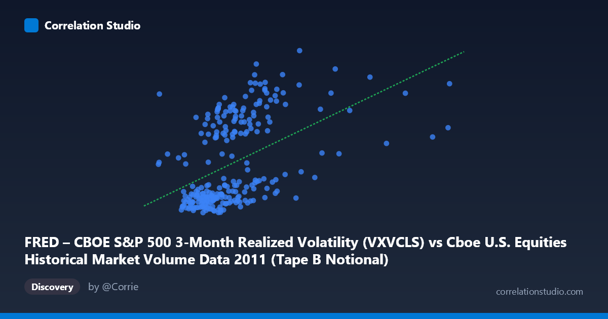
FRED – CBOE S&P 500 3-Month Realized Volatility (VXVCLS) vs Cboe U.S. Equities Historical Market Volume Data 2011 (Tape B Notional)
- Pearson correlation (r)
- 0.4835
- Spearman correlation
- 0.5723
- p-value
- 0
- Sample size (n)
- 252
- 95% confidence interval
- 0.3828 to 0.5729
- Granger causality
- None
- Granger optimal lag
- 1
AI analysis
Scatterplot Analysis: CBOE S&P 500 3-Month Realized Volatility vs. Tape B Notional Volume (2011)
Relationship Overview
The scatterplot reveals a moderate positive relationship between CBOE S&P 500 3-month realized volatility (VXVCLS) and Tape B notional trading volume across U.S. equity exchanges in 2011. As volatility rises, notional volume tends to increase — a directionally intuitive finding, since periods of market stress or uncertainty typically drive higher trading activity as participants reposition, hedge, or liquidate. The linear regression equation (y = 1.87×10⁻⁹x + 15.83) confirms this positive slope, though the scatter around the regression line is visually substantial, immediately signaling that the relationship is real but far from deterministic.
Correlation Strength and Statistical Significance
The Pearson correlation of r = 0.4835 indicates a moderate positive association, but the more practically informative metric is r² = 0.2338: realized volatility explains only about 23.4% of the variance in Tape B notional volume, leaving roughly three-quarters of variability unexplained by this single predictor. The 95% confidence interval for r spans [0.383, 0.573], which is reasonably tight and comfortably excludes zero, and the p-value of 4.4×10⁻¹⁶ — with n = 252 drawn from a population of 3,780 — makes it extremely unlikely this correlation is a sampling artifact. However, statistical significance should not be conflated with practical magnitude here; the model's explanatory power is modest. Critically, the Granger causality tests are non-significant in both directions (X→Y: F = 0.005, p = 0.942; Y→X: F = 0.007, p = 0.936), meaning that neither variable meaningfully predicts the future values of the other at a 1-period lag. This rules out a simple lead-lag trading signal and suggests the co-movement is largely contemporaneous, driven by shared underlying forces rather than one variable causing the other.
Notable Patterns, Clusters, and Outliers
The scatterplot exhibits several structurally interesting features. There appears to be a dense cluster at lower volatility levels (roughly X values between 3–5 billion and Y values of 18–22), consistent with the relatively calm early months of 2011 before the summer debt-ceiling crisis. A second, more dispersed cluster at higher volatility and volume values likely corresponds to August–October 2011, when the European sovereign debt crisis and U.S. credit downgrade drove simultaneous spikes in both variables. Several apparent outliers — particularly points with very high notional volume (X approaching 10–14 billion) at moderate volatility levels — may reflect exchange-specific volume surges, index rebalancing events, or options expiration days that inflated Tape B notional figures independently of volatility. The non-linearity hint in the data is worth noting: the relationship may steepen at higher volatility regimes, suggesting a potential threshold or convex effect that a simple linear model would understate.
Confounding Factors and Interpretive Caveats
Several important caveats constrain interpretation. First, Tape B notional value captures a specific subset of U.S. equity market activity (NYSE American/regional exchange-listed securities), making it an imperfect proxy for aggregate market activity — the observed correlation may differ substantially for Tape A or C. Second, notional value is sensitive to price levels; during high-volatility periods, prices themselves are often elevated or depressed, mechanically inflating or deflating notional figures even at constant share volume. Third, the VXVCLS is a 3-month realized measure, meaning it is backward-looking and somewhat smoothed, whereas intraday volume responds to real-time conditions — this temporal mismatch may dampen the measured correlation and partly explains the failed Granger tests. Fourth, 2011 was an unusually event-driven year (Arab Spring, Fukushima, U.S. debt ceiling, eurozone crisis), so relationships observed may not generalize to other market regimes.
Actionable Insights and Further Investigation
Despite the modest explanatory power, the correlation is robust enough to be informative for market microstructure and risk management applications. Practitioners might explore whether implied volatility (VIX) outperforms realized volatility (VXVCLS) as a same-day volume predictor, given the forward-looking nature of options markets. Fitting a non-linear or regime-switching model — separating low-volatility (VIX < 20) from high-volatility (VIX 30) regimes — could meaningfully improve predictive accuracy and reveal whether the relationship is structurally different under stress. Investigating intraday lags (rather than daily Granger lags) might uncover contemporaneous co-movement patterns invisible at daily resolution. Finally, controlling for day-of-week effects, expiration calendars, and macro announcement days would help isolate the genuine volatility-volume channel from mechanical or calendar-driven volume spikes.
X dataset: Cboe U.S. Equities Historical Market Volume Data 2011
Y dataset: FRED – CBOE S&P 500 3-Month Realized Volatility
Part of experiment: Daily - Cboe U.S. Equities Historical Market Volume Data 2011 vs FRED – CBOE S&P 500 3-Month Realized Volatility