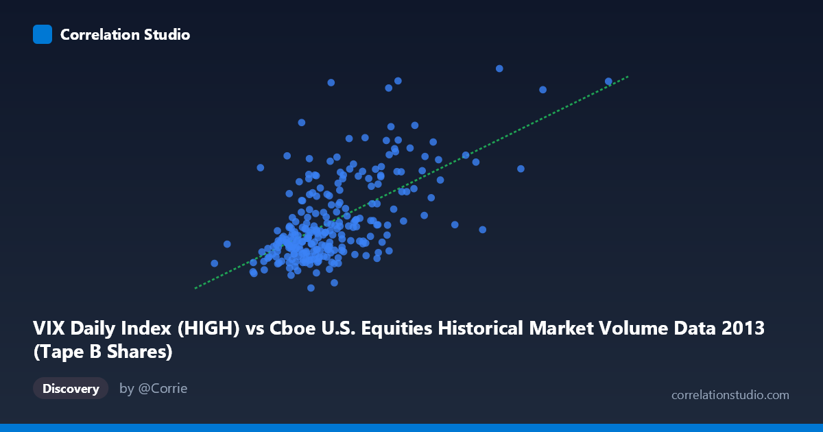
VIX Daily Index (HIGH) vs Cboe U.S. Equities Historical Market Volume Data 2013 (Tape B Shares)
- Pearson correlation (r)
- 0.6117
- Spearman correlation
- 0.5494
- p-value
- 0
- Sample size (n)
- 252
- 95% confidence interval
- 0.5281 to 0.6836
- Granger causality
- None
- Granger optimal lag
- 1
AI analysis
Scatterplot Analysis: VIX Daily Index (HIGH) vs. Tape B Shares (2013)
Relationship Overview The scatterplot reveals a moderate positive relationship between the VIX Daily Index High values and Cboe U.S. Equities Tape B share volume for 2013. As VIX levels increase, Tape B share volume tends to rise correspondingly, which aligns with well-established market intuition: elevated volatility typically drives higher trading activity as investors rebalance, hedge, or react to uncertainty. The linear regression equation (y = 6.63e-8x + 10.16) confirms this upward slope, though the substantial scatter around the regression line makes clear that this is far from a deterministic relationship. The data spans the full 2013 calendar year (N=3,780 population; n=252 paired samples), providing reasonably broad temporal coverage.
Correlation Strength and Statistical Significance The Pearson correlation of r = 0.611 indicates a moderate positive association, but the more informative statistic is r² = 0.374, meaning that VIX High values explain only about 37.4% of the variance in Tape B share volume — leaving roughly 62.6% unexplained by this relationship alone. The 95% confidence interval [0.528, 0.684] is relatively tight and does not cross zero, and the p-value of effectively 0 confirms this correlation is highly statistically significant given the sample size. However, statistical significance should not be conflated with practical or causal significance. Notably, Granger causality tests reveal no significant predictive directionality in either direction (X→Y: F=0.71, p=0.40; Y→X: F=0.07, p=0.79), meaning that past VIX values do not reliably predict future Tape B volume and vice versa at a 1-period lag. This important finding suggests the correlation is likely contemporaneous rather than predictive, limiting its utility for forecasting.
Notable Patterns, Clusters, and Outliers The sample points reveal several noteworthy features in the data distribution. The bulk of observations cluster in the X range of roughly 55–95 million (VIX High) with Y values between approximately 12.5–17, forming a reasonably dense core. However, there are several visible outliers that deserve attention: the point near (70.2M, 21.26) and (89.9M, 21.01) represent anomalously high Tape B volume relative to the broader pattern, suggesting specific market events drove unusual activity. Similarly, the point at (119.7M, 17.58) and (135.0M, 17.27) sit at the far right of the X distribution, representing extreme VIX High days — yet their Y values are not proportionally extreme, potentially indicating a non-linear or ceiling effect at very high volatility levels. The scatter also appears to widen at higher X values, hinting at heteroscedasticity (increasing variance as VIX rises).
Confounding Factors and Caveats Several important caveats limit straightforward interpretation of this correlation. First, the axes appear to be swapped relative to conventional expectation: the X-axis is labeled as VIX High (a volatility index, typically a smaller-scale number like 11–25) yet shows values in the tens of millions, while the Y-axis labeled as Tape B Shares shows values in the 12–22 range — suggesting possible metadata labeling inconsistency that warrants verification before drawing firm conclusions. Assuming the data is correctly mapped, both VIX and equity volume are jointly driven by common macro factors such as earnings seasons, Federal Reserve announcements, geopolitical events, and end-of-quarter rebalancing — making it difficult to disentangle direct causality from shared external drivers. Additionally, 2013 was a particularly low-volatility bull market year, which may limit the generalizability of these findings to periods of market stress.
Actionable Insights and Further Investigation Given the moderate correlation and absence of Granger causality, practitioners should be cautious about using VIX levels alone as a predictive signal for Tape B volume. Several follow-up analyses are recommended: (1) Investigate the identified outlier points (particularly those with Y 20) to determine whether specific market events (e.g., taper tantrum in May-June 2013) explain the anomalies; (2) Test non-linear regression models (e.g., logarithmic or polynomial) to check whether they better capture the apparent heteroscedasticity and potential ceiling effects at extreme VIX values; (3) Introduce lagged variables beyond 1 period and control for known confounders (day-of-week effects, earnings calendar, macro announcements) to build a more robust multivariate model; and (4) Verify the axis metadata to ensure variables are correctly assigned, as the scale discrepancy between labels and values raises data quality concerns that could materially affect all downstream conclusions.
X dataset: Cboe U.S. Equities Historical Market Volume Data 2013
Y dataset: VIX Daily Index
Part of experiment: Daily - Cboe U.S. Equities Historical Market Volume Data 2013 vs VIX Daily Index